pacman::p_load(sf, tmap, tidyverse, gtsummary)1 Overview
Thematic mapping involves the use of map symbols to visualize selected properties of geographic features that are not naturally visible, such as population, temperature, crime rate, and property prices, just to mention a few of them.
Geovisualisation, on the other hand, works by providing graphical ideation to render a place, a phenomenon or a process visible, enabling human’s most powerful information-processing abilities – those of spatial cognition associated with our eye–brain vision system – to be directly brought to bear.
Choropleth mapping involves the symbolisation of enumeration units, such as countries, provinces, states, counties or census units, using area patterns or graduated colors. For example, a social scientist may need to use a choropleth map to portray the spatial distribution of aged population of Singapore by Master Plan 2014 Subzone Boundary.
In this chapter, we learn how to plot functional and truthful choropleth maps by using an R package called tmap package.
2 The Packages
| Package | Description |
|---|---|
| tidyverse | A collection of functions for performing data science task such as importing, tidying, wrangling data and visualising data. In particular: |
| sf | For importing, managing, and processing geospatial data. |
| tmap | For thematic mapping |
| gtsummary | For summary and analytical tables |
The code chunk below will be used to install and load these packages in RStudio.
3 The Data
| Type | Details | Screenshot |
|---|---|---|
| Geospatial | Master Plan 2014 Subzone Boundary Web Consists of the geographical boundary of Singapore at the planning subzone level. The data is based on URA Master Plan 2014. Source: data.gov.sg |
|
| Aspatial | Singapore Residents by Planning Area / Subzone, Age Group, Sex and Type of Dwelling, June 2011-2020 Although it does not contain any coordinates values, but it’s PA and SZ fields can be used as unique identifiers to geocode to MP14_SUBZONE_WEB_PL shapefile. Source: singstat.gov.sg |
The code chunk below uses the st_read() function of sf package to import MP14_SUBZONE_WEB_PL shapefile as a simple feature data frame called mpsz.
mpsz <- st_read(dsn="data/geospatial",
                layer = "MP14_SUBZONE_WEB_PL")
Reading layer `MP14_SUBZONE_WEB_PL' from data source
`C:\kytjy\ISSS626-GAA\Hands-on_Ex\Hands-on_Ex01\data\geospatial'
using driver `ESRI Shapefile'
Simple feature collection with 323 features and 15 fields
Geometry type: MULTIPOLYGON
Dimension: XY
Bounding box: xmin: 2667.538 ymin: 15748.72 xmax: 56396.44 ymax: 50256.33
Projected CRS: SVY21Examine the content of mpsz by using the code chunk below:
glimpse(mpsz)Rows: 323
Columns: 16
$ OBJECTID <int> 1, 2, 3, 4, 5, 6, 7, 8, 9, 10, 11, 12, 13, 14, 15, 16, 17, …
$ SUBZONE_NO <int> 1, 1, 3, 8, 3, 7, 9, 2, 13, 7, 12, 6, 1, 5, 1, 1, 3, 2, 2, …
$ SUBZONE_N <chr> "MARINA SOUTH", "PEARL'S HILL", "BOAT QUAY", "HENDERSON HIL…
$ SUBZONE_C <chr> "MSSZ01", "OTSZ01", "SRSZ03", "BMSZ08", "BMSZ03", "BMSZ07",…
$ CA_IND <chr> "Y", "Y", "Y", "N", "N", "N", "N", "Y", "N", "N", "N", "N",…
$ PLN_AREA_N <chr> "MARINA SOUTH", "OUTRAM", "SINGAPORE RIVER", "BUKIT MERAH",…
$ PLN_AREA_C <chr> "MS", "OT", "SR", "BM", "BM", "BM", "BM", "SR", "QT", "QT",…
$ REGION_N <chr> "CENTRAL REGION", "CENTRAL REGION", "CENTRAL REGION", "CENT…
$ REGION_C <chr> "CR", "CR", "CR", "CR", "CR", "CR", "CR", "CR", "CR", "CR",…
$ INC_CRC <chr> "5ED7EB253F99252E", "8C7149B9EB32EEFC", "C35FEFF02B13E0E5",…
$ FMEL_UPD_D <date> 2014-12-05, 2014-12-05, 2014-12-05, 2014-12-05, 2014-12-05…
$ X_ADDR <dbl> 31595.84, 28679.06, 29654.96, 26782.83, 26201.96, 25358.82,…
$ Y_ADDR <dbl> 29220.19, 29782.05, 29974.66, 29933.77, 30005.70, 29991.38,…
$ SHAPE_Leng <dbl> 5267.381, 3506.107, 1740.926, 3313.625, 2825.594, 4428.913,…
$ SHAPE_Area <dbl> 1630379.27, 559816.25, 160807.50, 595428.89, 387429.44, 103…
$ geometry <MULTIPOLYGON [m]> MULTIPOLYGON (((31495.56 30..., MULTIPOLYGON (…mpszSimple feature collection with 323 features and 15 fields
Geometry type: MULTIPOLYGON
Dimension: XY
Bounding box: xmin: 2667.538 ymin: 15748.72 xmax: 56396.44 ymax: 50256.33
Projected CRS: SVY21
First 10 features:
OBJECTID SUBZONE_NO SUBZONE_N SUBZONE_C CA_IND PLN_AREA_N
1 1 1 MARINA SOUTH MSSZ01 Y MARINA SOUTH
2 2 1 PEARL'S HILL OTSZ01 Y OUTRAM
3 3 3 BOAT QUAY SRSZ03 Y SINGAPORE RIVER
4 4 8 HENDERSON HILL BMSZ08 N BUKIT MERAH
5 5 3 REDHILL BMSZ03 N BUKIT MERAH
6 6 7 ALEXANDRA HILL BMSZ07 N BUKIT MERAH
7 7 9 BUKIT HO SWEE BMSZ09 N BUKIT MERAH
8 8 2 CLARKE QUAY SRSZ02 Y SINGAPORE RIVER
9 9 13 PASIR PANJANG 1 QTSZ13 N QUEENSTOWN
10 10 7 QUEENSWAY QTSZ07 N QUEENSTOWN
PLN_AREA_C REGION_N REGION_C INC_CRC FMEL_UPD_D X_ADDR
1 MS CENTRAL REGION CR 5ED7EB253F99252E 2014-12-05 31595.84
2 OT CENTRAL REGION CR 8C7149B9EB32EEFC 2014-12-05 28679.06
3 SR CENTRAL REGION CR C35FEFF02B13E0E5 2014-12-05 29654.96
4 BM CENTRAL REGION CR 3775D82C5DDBEFBD 2014-12-05 26782.83
5 BM CENTRAL REGION CR 85D9ABEF0A40678F 2014-12-05 26201.96
6 BM CENTRAL REGION CR 9D286521EF5E3B59 2014-12-05 25358.82
7 BM CENTRAL REGION CR 7839A8577144EFE2 2014-12-05 27680.06
8 SR CENTRAL REGION CR 48661DC0FBA09F7A 2014-12-05 29253.21
9 QT CENTRAL REGION CR 1F721290C421BFAB 2014-12-05 22077.34
10 QT CENTRAL REGION CR 3580D2AFFBEE914C 2014-12-05 24168.31
Y_ADDR SHAPE_Leng SHAPE_Area geometry
1 29220.19 5267.381 1630379.3 MULTIPOLYGON (((31495.56 30...
2 29782.05 3506.107 559816.2 MULTIPOLYGON (((29092.28 30...
3 29974.66 1740.926 160807.5 MULTIPOLYGON (((29932.33 29...
4 29933.77 3313.625 595428.9 MULTIPOLYGON (((27131.28 30...
5 30005.70 2825.594 387429.4 MULTIPOLYGON (((26451.03 30...
6 29991.38 4428.913 1030378.8 MULTIPOLYGON (((25899.7 297...
7 30230.86 3275.312 551732.0 MULTIPOLYGON (((27746.95 30...
8 30222.86 2208.619 290184.7 MULTIPOLYGON (((29351.26 29...
9 29893.78 6571.323 1084792.3 MULTIPOLYGON (((20996.49 30...
10 30104.18 3454.239 631644.3 MULTIPOLYGON (((24472.11 29...Next, we will import respopagsex2000to2018.csv file into RStudio and save the file into an R dataframe called popdata. The task will be performed by using read_csv() function of readr package.
popdata <- read_csv("data/aspatial/respopagesextod2011to2020.csv")| Characteristic | N | N = 984,6561 |
|---|---|---|
| PA | 984,656 | |
| Ang Mo Kio | 36,480 (3.7%) | |
| Bedok | 24,320 (2.5%) | |
| Bishan | 9,120 (0.9%) | |
| Boon Lay | 12,160 (1.2%) | |
| Bukit Batok | 27,360 (2.8%) | |
| Bukit Merah | 51,680 (5.2%) | |
| Bukit Panjang | 21,280 (2.2%) | |
| Bukit Timah | 24,320 (2.5%) | |
| Central Water Catchment | 3,040 (0.3%) | |
| Changi | 9,120 (0.9%) | |
| Changi Bay | 3,040 (0.3%) | |
| Choa Chu Kang | 18,240 (1.9%) | |
| Clementi | 27,360 (2.8%) | |
| Downtown Core | 36,784 (3.7%) | |
| Geylang | 15,200 (1.5%) | |
| Hougang | 30,400 (3.1%) | |
| Jurong East | 30,704 (3.1%) | |
| Jurong West | 27,360 (2.8%) | |
| Kallang | 27,360 (2.8%) | |
| Lim Chu Kang | 3,040 (0.3%) | |
| Mandai | 9,120 (0.9%) | |
| Marina East | 3,040 (0.3%) | |
| Marina South | 3,040 (0.3%) | |
| Marine Parade | 15,200 (1.5%) | |
| Museum | 9,120 (0.9%) | |
| Newton | 18,240 (1.9%) | |
| North-Eastern Islands | 3,040 (0.3%) | |
| Novena | 15,200 (1.5%) | |
| Orchard | 9,120 (0.9%) | |
| Outram | 12,160 (1.2%) | |
| Pasir Ris | 24,320 (2.5%) | |
| Paya Lebar | 15,200 (1.5%) | |
| Pioneer | 15,200 (1.5%) | |
| Punggol | 21,280 (2.2%) | |
| Queenstown | 45,600 (4.6%) | |
| River Valley | 15,200 (1.5%) | |
| Rochor | 30,400 (3.1%) | |
| Seletar | 12,160 (1.2%) | |
| Sembawang | 27,360 (2.8%) | |
| Sengkang | 21,280 (2.2%) | |
| Serangoon | 21,280 (2.2%) | |
| Simpang | 12,160 (1.2%) | |
| Singapore River | 9,120 (0.9%) | |
| Southern Islands | 6,080 (0.6%) | |
| Straits View | 3,040 (0.3%) | |
| Sungei Kadut | 15,200 (1.5%) | |
| Tampines | 15,200 (1.5%) | |
| Tanglin | 12,160 (1.2%) | |
| Tengah | 4,560 (0.5%) | |
| Toa Payoh | 36,480 (3.7%) | |
| Tuas | 18,240 (1.9%) | |
| Western Islands | 9,120 (0.9%) | |
| Western Water Catchment | 3,648 (0.4%) | |
| Woodlands | 27,360 (2.8%) | |
| Yishun | 27,360 (2.8%) | |
| SZ | 984,656 | |
| Admiralty | 3,040 (0.3%) | |
| Airport Road | 3,040 (0.3%) | |
| Alexandra Hill | 3,040 (0.3%) | |
| Alexandra North | 3,040 (0.3%) | |
| Aljunied | 3,040 (0.3%) | |
| Anak Bukit | 3,040 (0.3%) | |
| Anchorvale | 3,040 (0.3%) | |
| Ang Mo Kio Town Centre | 3,040 (0.3%) | |
| Anson | 3,040 (0.3%) | |
| Bahar | 304 (<0.1%) | |
| Balestier | 3,040 (0.3%) | |
| Bangkit | 3,040 (0.3%) | |
| Bayfront Subzone | 3,040 (0.3%) | |
| Bayshore | 3,040 (0.3%) | |
| Bedok North | 3,040 (0.3%) | |
| Bedok Reservoir | 3,040 (0.3%) | |
| Bedok South | 3,040 (0.3%) | |
| Bencoolen | 3,040 (0.3%) | |
| Bendemeer | 3,040 (0.3%) | |
| Benoi Sector | 3,040 (0.3%) | |
| Bidadari | 3,040 (0.3%) | |
| Bishan East | 3,040 (0.3%) | |
| Boat Quay | 3,040 (0.3%) | |
| Boon Keng | 3,040 (0.3%) | |
| Boon Lay Place | 3,040 (0.3%) | |
| Boon Teck | 3,040 (0.3%) | |
| Boulevard | 3,040 (0.3%) | |
| Braddell | 3,040 (0.3%) | |
| Bras Basah | 3,040 (0.3%) | |
| Brickland | 304 (<0.1%) | |
| Brickworks | 3,040 (0.3%) | |
| Bugis | 3,040 (0.3%) | |
| Bukit Batok Central | 3,040 (0.3%) | |
| Bukit Batok East | 3,040 (0.3%) | |
| Bukit Batok South | 3,040 (0.3%) | |
| Bukit Batok West | 3,040 (0.3%) | |
| Bukit Ho Swee | 3,040 (0.3%) | |
| Bukit Merah | 3,040 (0.3%) | |
| Cairnhill | 3,040 (0.3%) | |
| Cecil | 3,040 (0.3%) | |
| Central Subzone | 3,040 (0.3%) | |
| Central Water Catchment | 3,040 (0.3%) | |
| Changi Airport | 3,040 (0.3%) | |
| Changi Bay | 3,040 (0.3%) | |
| Changi Point | 3,040 (0.3%) | |
| Changi West | 3,040 (0.3%) | |
| Chatsworth | 3,040 (0.3%) | |
| Cheng San | 3,040 (0.3%) | |
| Chin Bee | 3,040 (0.3%) | |
| China Square | 3,040 (0.3%) | |
| Chinatown | 3,040 (0.3%) | |
| Choa Chu Kang Central | 3,040 (0.3%) | |
| Choa Chu Kang North | 3,040 (0.3%) | |
| Chong Boon | 3,040 (0.3%) | |
| City Hall | 3,040 (0.3%) | |
| City Terminals | 3,040 (0.3%) | |
| Clarke Quay | 3,040 (0.3%) | |
| Cleantech | 304 (<0.1%) | |
| Clementi Central | 3,040 (0.3%) | |
| Clementi North | 3,040 (0.3%) | |
| Clementi West | 3,040 (0.3%) | |
| Clementi Woods | 3,040 (0.3%) | |
| Clifford Pier | 3,040 (0.3%) | |
| Commonwealth | 3,040 (0.3%) | |
| Compassvale | 3,040 (0.3%) | |
| Coney Island | 3,040 (0.3%) | |
| Coronation Road | 3,040 (0.3%) | |
| Crawford | 3,040 (0.3%) | |
| Dairy Farm | 3,040 (0.3%) | |
| Defu Industrial Park | 3,040 (0.3%) | |
| Depot Road | 3,040 (0.3%) | |
| Dhoby Ghaut | 3,040 (0.3%) | |
| Dover | 3,040 (0.3%) | |
| Dunearn | 3,040 (0.3%) | |
| East Coast | 3,040 (0.3%) | |
| Everton Park | 3,040 (0.3%) | |
| Faber | 3,040 (0.3%) | |
| Fajar | 3,040 (0.3%) | |
| Farrer Court | 3,040 (0.3%) | |
| Farrer Park | 3,040 (0.3%) | |
| Fernvale | 3,040 (0.3%) | |
| Flora Drive | 3,040 (0.3%) | |
| Forest Hill | 304 (<0.1%) | |
| Fort Canning | 3,040 (0.3%) | |
| Frankel | 3,040 (0.3%) | |
| Gali Batu | 3,040 (0.3%) | |
| Garden | 304 (<0.1%) | |
| Geylang Bahru | 3,040 (0.3%) | |
| Geylang East | 3,040 (0.3%) | |
| Ghim Moh | 3,040 (0.3%) | |
| Gombak | 3,040 (0.3%) | |
| Goodwood Park | 3,040 (0.3%) | |
| Greenwood Park | 3,040 (0.3%) | |
| Guilin | 3,040 (0.3%) | |
| Gul Basin | 3,040 (0.3%) | |
| Gul Circle | 3,040 (0.3%) | |
| Henderson Hill | 3,040 (0.3%) | |
| Hillcrest | 3,040 (0.3%) | |
| Hillview | 3,040 (0.3%) | |
| Holland Drive | 3,040 (0.3%) | |
| Holland Road | 3,040 (0.3%) | |
| Hong Kah | 3,040 (0.3%) | |
| Hong Kah North | 3,040 (0.3%) | |
| Hougang Central | 3,040 (0.3%) | |
| Hougang East | 3,040 (0.3%) | |
| Hougang West | 3,040 (0.3%) | |
| Institution Hill | 3,040 (0.3%) | |
| International Business Park | 3,040 (0.3%) | |
| Istana Negara | 3,040 (0.3%) | |
| Jelebu | 3,040 (0.3%) | |
| Joo Koon | 3,040 (0.3%) | |
| Joo Seng | 3,040 (0.3%) | |
| Jurong Gateway | 3,040 (0.3%) | |
| Jurong Island And Bukom | 3,040 (0.3%) | |
| Jurong Port | 3,040 (0.3%) | |
| Jurong River | 3,040 (0.3%) | |
| Jurong West Central | 3,040 (0.3%) | |
| Kaki Bukit | 3,040 (0.3%) | |
| Kallang Bahru | 3,040 (0.3%) | |
| Kallang Way | 3,040 (0.3%) | |
| Kampong Bugis | 3,040 (0.3%) | |
| Kampong Glam | 3,040 (0.3%) | |
| Kampong Java | 3,040 (0.3%) | |
| Kampong Tiong Bahru | 3,040 (0.3%) | |
| Kampong Ubi | 3,040 (0.3%) | |
| Kangkar | 3,040 (0.3%) | |
| Katong | 3,040 (0.3%) | |
| Keat Hong | 3,040 (0.3%) | |
| Kebun Bahru | 3,040 (0.3%) | |
| Kembangan | 3,040 (0.3%) | |
| Kent Ridge | 3,040 (0.3%) | |
| Khatib | 3,040 (0.3%) | |
| Kian Teck | 3,040 (0.3%) | |
| Kim Keat | 3,040 (0.3%) | |
| Kovan | 3,040 (0.3%) | |
| Kranji | 3,040 (0.3%) | |
| Lakeside | 2,736 (0.3%) | |
| Lakeside (Business) | 304 (<0.1%) | |
| Lakeside (Leisure) | 304 (<0.1%) | |
| Lavender | 3,040 (0.3%) | |
| Leedon Park | 3,040 (0.3%) | |
| Leonie Hill | 3,040 (0.3%) | |
| Lim Chu Kang | 3,040 (0.3%) | |
| Little India | 3,040 (0.3%) | |
| Liu Fang | 3,040 (0.3%) | |
| Lorong 8 Toa Payoh | 3,040 (0.3%) | |
| Lorong Ah Soo | 3,040 (0.3%) | |
| Lorong Chuan | 3,040 (0.3%) | |
| Lorong Halus | 3,040 (0.3%) | |
| Lorong Halus North | 3,040 (0.3%) | |
| Lower Seletar | 3,040 (0.3%) | |
| Loyang East | 3,040 (0.3%) | |
| Loyang West | 3,040 (0.3%) | |
| Mackenzie | 3,040 (0.3%) | |
| Macpherson | 3,040 (0.3%) | |
| Malcolm | 3,040 (0.3%) | |
| Mandai East | 3,040 (0.3%) | |
| Mandai Estate | 3,040 (0.3%) | |
| Mandai West | 3,040 (0.3%) | |
| Margaret Drive | 3,040 (0.3%) | |
| Marina Centre | 3,040 (0.3%) | |
| Marina East | 3,040 (0.3%) | |
| Marina East (Mp) | 3,040 (0.3%) | |
| Marina South | 3,040 (0.3%) | |
| Marine Parade | 3,040 (0.3%) | |
| Maritime Square | 3,040 (0.3%) | |
| Marymount | 3,040 (0.3%) | |
| Matilda | 3,040 (0.3%) | |
| Maxwell | 3,040 (0.3%) | |
| Mei Chin | 3,040 (0.3%) | |
| Midview | 3,040 (0.3%) | |
| Monk's Hill | 3,040 (0.3%) | |
| Moulmein | 3,040 (0.3%) | |
| Mount Emily | 3,040 (0.3%) | |
| Mount Pleasant | 3,040 (0.3%) | |
| Mountbatten | 3,040 (0.3%) | |
| Murai | 304 (<0.1%) | |
| Nassim | 3,040 (0.3%) | |
| National University Of S'pore | 3,040 (0.3%) | |
| Nature Reserve | 3,040 (0.3%) | |
| Nee Soon | 3,040 (0.3%) | |
| Newton Circus | 3,040 (0.3%) | |
| Nicoll | 304 (<0.1%) | |
| North-Eastern Islands | 3,040 (0.3%) | |
| North Coast | 3,040 (0.3%) | |
| Northland | 3,040 (0.3%) | |
| Northshore | 3,040 (0.3%) | |
| One North | 3,040 (0.3%) | |
| One Tree Hill | 3,040 (0.3%) | |
| Orange Grove | 3,040 (0.3%) | |
| Oxley | 3,040 (0.3%) | |
| Pandan | 3,040 (0.3%) | |
| Pang Sua | 3,040 (0.3%) | |
| Park | 304 (<0.1%) | |
| Pasir Panjang 1 | 3,040 (0.3%) | |
| Pasir Panjang 2 | 3,040 (0.3%) | |
| Pasir Ris Central | 3,040 (0.3%) | |
| Pasir Ris Drive | 3,040 (0.3%) | |
| Pasir Ris Park | 3,040 (0.3%) | |
| Pasir Ris Wafer Fab Park | 3,040 (0.3%) | |
| Pasir Ris West | 3,040 (0.3%) | |
| Paterson | 3,040 (0.3%) | |
| Paya Lebar East | 3,040 (0.3%) | |
| Paya Lebar North | 3,040 (0.3%) | |
| Paya Lebar West | 3,040 (0.3%) | |
| Pearl's Hill | 3,040 (0.3%) | |
| Pei Chun | 3,040 (0.3%) | |
| Peng Siang | 3,040 (0.3%) | |
| Penjuru Crescent | 3,040 (0.3%) | |
| People's Park | 3,040 (0.3%) | |
| Phillip | 3,040 (0.3%) | |
| Pioneer Sector | 3,040 (0.3%) | |
| Plab | 3,040 (0.3%) | |
| Plantation | 304 (<0.1%) | |
| Port | 3,040 (0.3%) | |
| Potong Pasir | 3,040 (0.3%) | |
| Pulau Punggol Barat | 3,040 (0.3%) | |
| Pulau Punggol Timor | 3,040 (0.3%) | |
| Pulau Seletar | 3,040 (0.3%) | |
| Punggol Canal | 3,040 (0.3%) | |
| Punggol Field | 3,040 (0.3%) | |
| Punggol Town Centre | 3,040 (0.3%) | |
| Queensway | 3,040 (0.3%) | |
| Raffles Place | 3,040 (0.3%) | |
| Redhill | 3,040 (0.3%) | |
| Reservoir View | 3,040 (0.3%) | |
| Ridout | 3,040 (0.3%) | |
| Rivervale | 3,040 (0.3%) | |
| Robertson Quay | 3,040 (0.3%) | |
| Rochor Canal | 3,040 (0.3%) | |
| Safti | 3,040 (0.3%) | |
| Samulun | 3,040 (0.3%) | |
| Saujana | 3,040 (0.3%) | |
| Selegie | 3,040 (0.3%) | |
| Seletar | 3,040 (0.3%) | |
| Seletar Aerospace Park | 3,040 (0.3%) | |
| Seletar Hills | 3,040 (0.3%) | |
| Semakau | 3,040 (0.3%) | |
| Sembawang Central | 3,040 (0.3%) | |
| Sembawang East | 3,040 (0.3%) | |
| Sembawang Hills | 3,040 (0.3%) | |
| Sembawang North | 3,040 (0.3%) | |
| Sembawang Springs | 3,040 (0.3%) | |
| Sembawang Straits | 3,040 (0.3%) | |
| Sengkang Town Centre | 3,040 (0.3%) | |
| Sengkang West | 3,040 (0.3%) | |
| Senja | 3,040 (0.3%) | |
| Sennett | 3,040 (0.3%) | |
| Senoko North | 3,040 (0.3%) | |
| Senoko South | 3,040 (0.3%) | |
| Senoko West | 3,040 (0.3%) | |
| Sentosa | 3,040 (0.3%) | |
| Serangoon Central | 3,040 (0.3%) | |
| Serangoon Garden | 3,040 (0.3%) | |
| Serangoon North | 3,040 (0.3%) | |
| Serangoon North Ind Estate | 3,040 (0.3%) | |
| Shangri-La | 3,040 (0.3%) | |
| Shipyard | 3,040 (0.3%) | |
| Siglap | 3,040 (0.3%) | |
| Simei | 3,040 (0.3%) | |
| Simpang North | 3,040 (0.3%) | |
| Simpang South | 3,040 (0.3%) | |
| Singapore General Hospital | 3,040 (0.3%) | |
| Singapore Polytechnic | 3,040 (0.3%) | |
| Somerset | 3,040 (0.3%) | |
| Southern Group | 3,040 (0.3%) | |
| Springleaf | 3,040 (0.3%) | |
| Straits View | 3,040 (0.3%) | |
| Sudong | 3,040 (0.3%) | |
| Sungei Road | 3,040 (0.3%) | |
| Sunset Way | 3,040 (0.3%) | |
| Swiss Club | 3,040 (0.3%) | |
| Tagore | 3,040 (0.3%) | |
| Tai Seng | 3,040 (0.3%) | |
| Taman Jurong | 3,040 (0.3%) | |
| Tampines East | 3,040 (0.3%) | |
| Tampines North | 3,040 (0.3%) | |
| Tampines West | 3,040 (0.3%) | |
| Tanglin | 3,040 (0.3%) | |
| Tanglin Halt | 3,040 (0.3%) | |
| Tanjong Irau | 3,040 (0.3%) | |
| Tanjong Pagar | 3,040 (0.3%) | |
| Tanjong Rhu | 3,040 (0.3%) | |
| Teban Gardens | 3,040 (0.3%) | |
| Teck Whye | 3,040 (0.3%) | |
| Telok Blangah Drive | 3,040 (0.3%) | |
| Telok Blangah Rise | 3,040 (0.3%) | |
| Telok Blangah Way | 3,040 (0.3%) | |
| Tengah | 2,736 (0.3%) | |
| Tengah Industrial Estate | 304 (<0.1%) | |
| Tengeh | 3,040 (0.3%) | |
| The Wharves | 3,040 (0.3%) | |
| Tiong Bahru | 3,040 (0.3%) | |
| Tiong Bahru Station | 3,040 (0.3%) | |
| Toa Payoh Central | 3,040 (0.3%) | |
| Toa Payoh West | 3,040 (0.3%) | |
| Toh Guan | 3,040 (0.3%) | |
| Toh Tuck | 3,040 (0.3%) | |
| Townsville | 3,040 (0.3%) | |
| Trafalgar | 3,040 (0.3%) | |
| Tuas Bay | 3,040 (0.3%) | |
| Tuas North | 3,040 (0.3%) | |
| Tuas Promenade | 3,040 (0.3%) | |
| Tuas View | 3,040 (0.3%) | |
| Tuas View Extension | 3,040 (0.3%) | |
| Tukang | 3,040 (0.3%) | |
| Turf Club | 3,040 (0.3%) | |
| Tyersall | 3,040 (0.3%) | |
| Ulu Pandan | 3,040 (0.3%) | |
| Upper Paya Lebar | 3,040 (0.3%) | |
| Upper Thomson | 3,040 (0.3%) | |
| Victoria | 3,040 (0.3%) | |
| Waterway East | 3,040 (0.3%) | |
| Wenya | 3,040 (0.3%) | |
| West Coast | 3,040 (0.3%) | |
| Western Water Catchment | 2,736 (0.3%) | |
| Woodgrove | 3,040 (0.3%) | |
| Woodlands East | 3,040 (0.3%) | |
| Woodlands Regional Centre | 3,040 (0.3%) | |
| Woodlands South | 3,040 (0.3%) | |
| Woodlands West | 3,040 (0.3%) | |
| Woodleigh | 3,040 (0.3%) | |
| Xilin | 3,040 (0.3%) | |
| Yew Tee | 3,040 (0.3%) | |
| Yio Chu Kang | 3,040 (0.3%) | |
| Yio Chu Kang East | 3,040 (0.3%) | |
| Yio Chu Kang North | 3,040 (0.3%) | |
| Yio Chu Kang West | 3,040 (0.3%) | |
| Yishun Central | 3,040 (0.3%) | |
| Yishun East | 3,040 (0.3%) | |
| Yishun South | 3,040 (0.3%) | |
| Yishun West | 3,040 (0.3%) | |
| Yuhua East | 3,040 (0.3%) | |
| Yuhua West | 3,040 (0.3%) | |
| Yunnan | 3,040 (0.3%) | |
| AG | 984,656 | |
| 0_to_4 | 51,824 (5.3%) | |
| 10_to_14 | 51,824 (5.3%) | |
| 15_to_19 | 51,824 (5.3%) | |
| 20_to_24 | 51,824 (5.3%) | |
| 25_to_29 | 51,824 (5.3%) | |
| 30_to_34 | 51,824 (5.3%) | |
| 35_to_39 | 51,824 (5.3%) | |
| 40_to_44 | 51,824 (5.3%) | |
| 45_to_49 | 51,824 (5.3%) | |
| 5_to_9 | 51,824 (5.3%) | |
| 50_to_54 | 51,824 (5.3%) | |
| 55_to_59 | 51,824 (5.3%) | |
| 60_to_64 | 51,824 (5.3%) | |
| 65_to_69 | 51,824 (5.3%) | |
| 70_to_74 | 51,824 (5.3%) | |
| 75_to_79 | 51,824 (5.3%) | |
| 80_to_84 | 51,824 (5.3%) | |
| 85_to_89 | 51,824 (5.3%) | |
| 90_and_over | 51,824 (5.3%) | |
| Sex | 984,656 | |
| Females | 492,328 (50%) | |
| Males | 492,328 (50%) | |
| TOD | 984,656 | |
| Condominiums and Other Apartments | 123,082 (13%) | |
| HDB 1- and 2-Room Flats | 123,082 (13%) | |
| HDB 3-Room Flats | 123,082 (13%) | |
| HDB 4-Room Flats | 123,082 (13%) | |
| HDB 5-Room and Executive Flats | 123,082 (13%) | |
| HUDC Flats (excluding those privatised) | 123,082 (13%) | |
| Landed Properties | 123,082 (13%) | |
| Others | 123,082 (13%) | |
| Pop | 984,656 | 0 (0, 10) |
| Time | 984,656 | 2,016.00 (2,013.00, 2,018.00) |
| 1 n (%); Median (IQR) | ||
4 Data Preparation
Before a thematic map can be prepared, we will need to prepare a data table with year 2020 values.
The data table should include the variables PA, SZ, YOUNG, ECONOMY ACTIVE, AGED, TOTAL, DEPENDENCY.
- YOUNG: age group 0 to 4 until age group 20 to 24,
- ECONOMY ACTIVE: age group 25-29 until age group 60-64,
- AGED: age group 65 and above,
- TOTAL: all age group, and
- DEPENDENCY: the ratio between young and aged against economy active group
4.1 Data Wrangling
The following data wrangling and transformation functions will be used:
pivot_wider()of tidyr package, andmutate(),filter(),group_by(), andselect()of dplyr package
popdata2020 <- popdata %>%
  filter(Time==2020) %>%
  group_by(PA, SZ, AG) %>% # Group by Planning Area, Subzone, Age Group
  summarise(`POP`=sum(`Pop`)) %>%  # Summarise by # of population
  ungroup() %>%
  pivot_wider(names_from=AG,
              values_from = POP)

colnames(popdata2020)
[1] "PA" "SZ" "0_to_4" "10_to_14" "15_to_19"
[6] "20_to_24" "25_to_29" "30_to_34" "35_to_39" "40_to_44"
[11] "45_to_49" "50_to_54" "55_to_59" "5_to_9" "60_to_64"
[16] "65_to_69" "70_to_74" "75_to_79" "80_to_84" "85_to_89"
[21] "90_and_over"popdata2020 <- popdata2020 %>%
# Young: Aged 0 to 24
mutate(YOUNG=rowSums(.[3:6]) # Aged 0 - 24, 10 - 24
+rowSums(.[14])) %>% # Aged 5 - 9
# Economic Active: Aged 25 to 64
mutate(`ECONOMY ACTIVE` = rowSums(.[7:13])+ # Aged 25 - 59
rowSums(.[15])) %>% # Aged 60 -64
# Aged: > 65
mutate(`AGED`=rowSums(.[16:21])) %>%
# Total: all age groups
mutate(`TOTAL`=rowSums(.[3:21])) %>%
# Proportion of inactive population per working population
mutate(`DEPENDENCY`=(`YOUNG` + `AGED`)
/ `ECONOMY ACTIVE`) %>%
select(`PA`, `SZ`, `YOUNG`,
`ECONOMY ACTIVE`, `AGED`,
`TOTAL`, `DEPENDENCY`)glimpse(popdata2020)Rows: 332
Columns: 7
$ PA <chr> "Ang Mo Kio", "Ang Mo Kio", "Ang Mo Kio", "Ang Mo Kio…
$ SZ <chr> "Ang Mo Kio Town Centre", "Cheng San", "Chong Boon", …
$ YOUNG <dbl> 1290, 5640, 5100, 4620, 1880, 3330, 1940, 4190, 0, 11…
$ `ECONOMY ACTIVE` <dbl> 2760, 16460, 15000, 13010, 3630, 9050, 4480, 11950, 0…
$ AGED <dbl> 760, 6050, 6470, 5120, 1310, 3610, 1530, 5100, 0, 750…
$ TOTAL <dbl> 4810, 28150, 26570, 22750, 6820, 15990, 7950, 21240, …
$ DEPENDENCY <dbl> 0.7427536, 0.7102066, 0.7713333, 0.7486549, 0.8787879…4.2 Joining the attribute data and geospatial data
Before we can perform the georelational join, one extra step is required to convert the values in PA and SZ fields to uppercase. This is because the values of PA and SZ fields are made up of upper- and lowercase. On the other, hand the SUBZONE_N and PLN_AREA_N are in uppercase.
popdata2020_upper <- popdata2020 %>%
  mutate_at(.vars=vars(PA, SZ),
            .funs=funs(toupper)) %>%
  filter(`ECONOMY ACTIVE` > 0)

class(popdata2020_upper)
[1] "tbl_df" "tbl" "data.frame"glimpse(popdata2020_upper)Rows: 234
Columns: 7
$ PA <chr> "ANG MO KIO", "ANG MO KIO", "ANG MO KIO", "ANG MO KIO…
$ SZ <chr> "ANG MO KIO TOWN CENTRE", "CHENG SAN", "CHONG BOON", …
$ YOUNG <dbl> 1290, 5640, 5100, 4620, 1880, 3330, 1940, 4190, 1110,…
$ `ECONOMY ACTIVE` <dbl> 2760, 16460, 15000, 13010, 3630, 9050, 4480, 11950, 2…
$ AGED <dbl> 760, 6050, 6470, 5120, 1310, 3610, 1530, 5100, 750, 4…
$ TOTAL <dbl> 4810, 28150, 26570, 22750, 6820, 15990, 7950, 21240, …
$ DEPENDENCY <dbl> 0.7427536, 0.7102066, 0.7713333, 0.7486549, 0.8787879…Next, left_join() of dplyr is used to join the geographical data and attribute table using planning subzone name e.g. SUBZONE_N and SZ as the common identifier.
left_join() of dplyr package is used with mpsz simple feature data frame as the left data table is to ensure that the output will be a simple features data frame.
mpsz_pop2020 <- left_join(mpsz, popdata2020_upper, # left: geospatial, right: aspatial
                  by = c("SUBZONE_N" = "SZ"))

class(mpsz_pop2020)
[1] "sf" "data.frame"write_rds() is used to save R object as RDS (R Data Serialization) format. RDS allows the preservation of the state of R objects between R sessions.
write_rds(mpsz_pop2020, "data/rds/mpszpop2020.rds")mpsz_pop2020 <- read_rds("data/rds/mpszpop2020.rds")5 Choropleth Mapping Geospatial Data Using tmap
Two approaches can be used to prepare thematic map using tmap, they are:
- Plotting a thematic map quickly by using
qtm(). - Plotting highly customisable thematic map by using tmap elements.
5.1 Plotting a choropleth map quickly by using qtm()
qtm():
- Easiest and quickest to draw a choropleth map using tmap
- Concise and provides a good default visualisation in many cases.
The code chunk below will draw a cartographic standard choropleth map as shown below.
tmap_mode("plot")

qtm(mpsz_pop2020,
    fill="DEPENDENCY")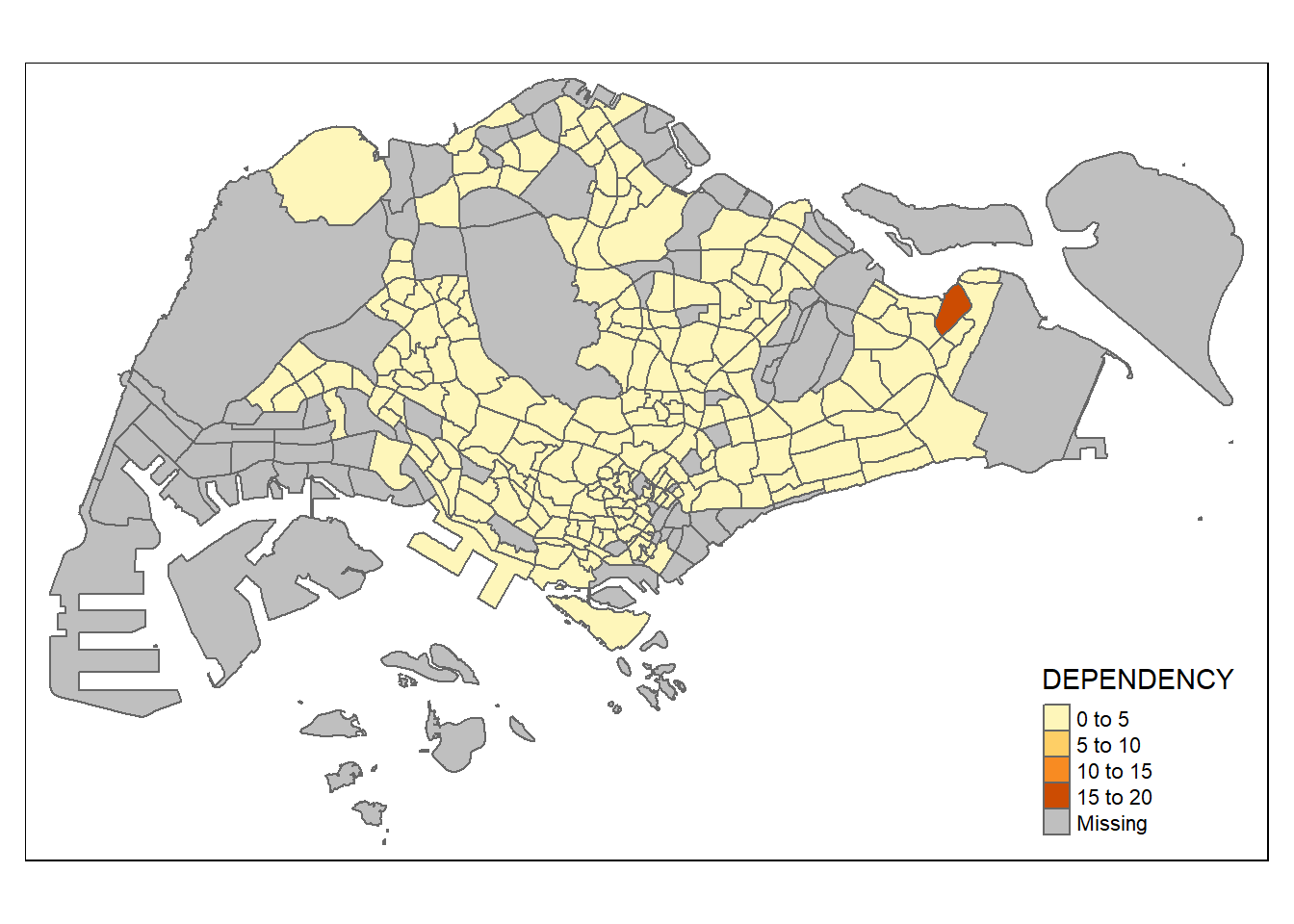
Note
tmap_mode()with plot option: used to produce a static map. For interactive mode, view option should be used.fillargument: is used to map the attribute (i.e. DEPENDENCY)
5.2 Creating a choropleth map by using tmap’s elements
Despite its usefulness of drawing a choropleth map quickly and easily, the disadvantge of qtm() is that it makes aesthetics of individual layers harder to control. To draw a high quality cartographic choropleth map as shown in the figure below, tmap’s drawing elements should be used.
tm_shape(mpsz_pop2020)+

  tm_fill("DEPENDENCY",
          style = "quantile",
          palette = "Blues",
          title = "Dependency ratio") +

  tm_layout(main.title = "Distribution of Dependency Ratio by planning subzone",
            main.title.position = "center",
            main.title.size = 1,
            legend.title.size = 1,
            legend.height = 0.45,
            legend.width = 0.35,
            bg.color = "#E4D5C9",
            frame = F) +

  tm_borders(alpha = 0.5) +
  tm_compass(type="8star", size = 1.5) +
  tm_scale_bar() +
  tm_grid(alpha =0.2) +
  tm_credits("Source: Planning Sub-zone boundary from Urban Redevelopment Authorithy (URA)\n and Population data from Department of Statistics (DOS)",
             position = c("left", "bottom"))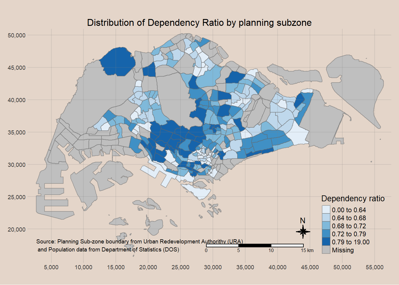
In the following sub-section, we will share with you tmap functions that used to plot these elements.
5.2.1 Drawing a base map
The basic building block of tmap is tm_shape() followed by one or more layer elemments such as tm_fill() and tm_polygons().
In the code chunk below, tm_shape() is used to define the input data (i.e mpsz_pop2020) and tm_polygons() is used to draw the planning subzone polygons.
tm_shape(mpsz_pop2020) +
  tm_polygons() + # for borders of the polygon
  tm_layout(bg.color = "#E4D5C9",
            frame = F)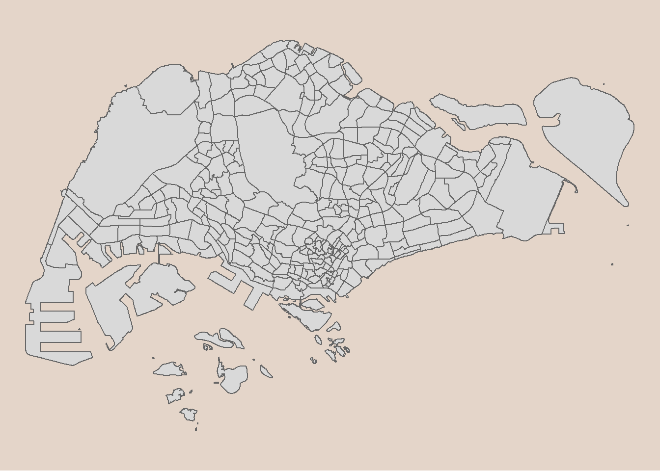
5.2.2 Drawing a choropleth map using tm_polygons()
To draw a choropleth map showing the geographical distribution of a selected variable by planning subzone, we just need to assign the target variable such as Dependency to tm_polygons().
tm_shape(mpsz_pop2020)+
  tm_polygons("DEPENDENCY") +
  tm_layout(bg.color = "#E4D5C9",
            frame = F)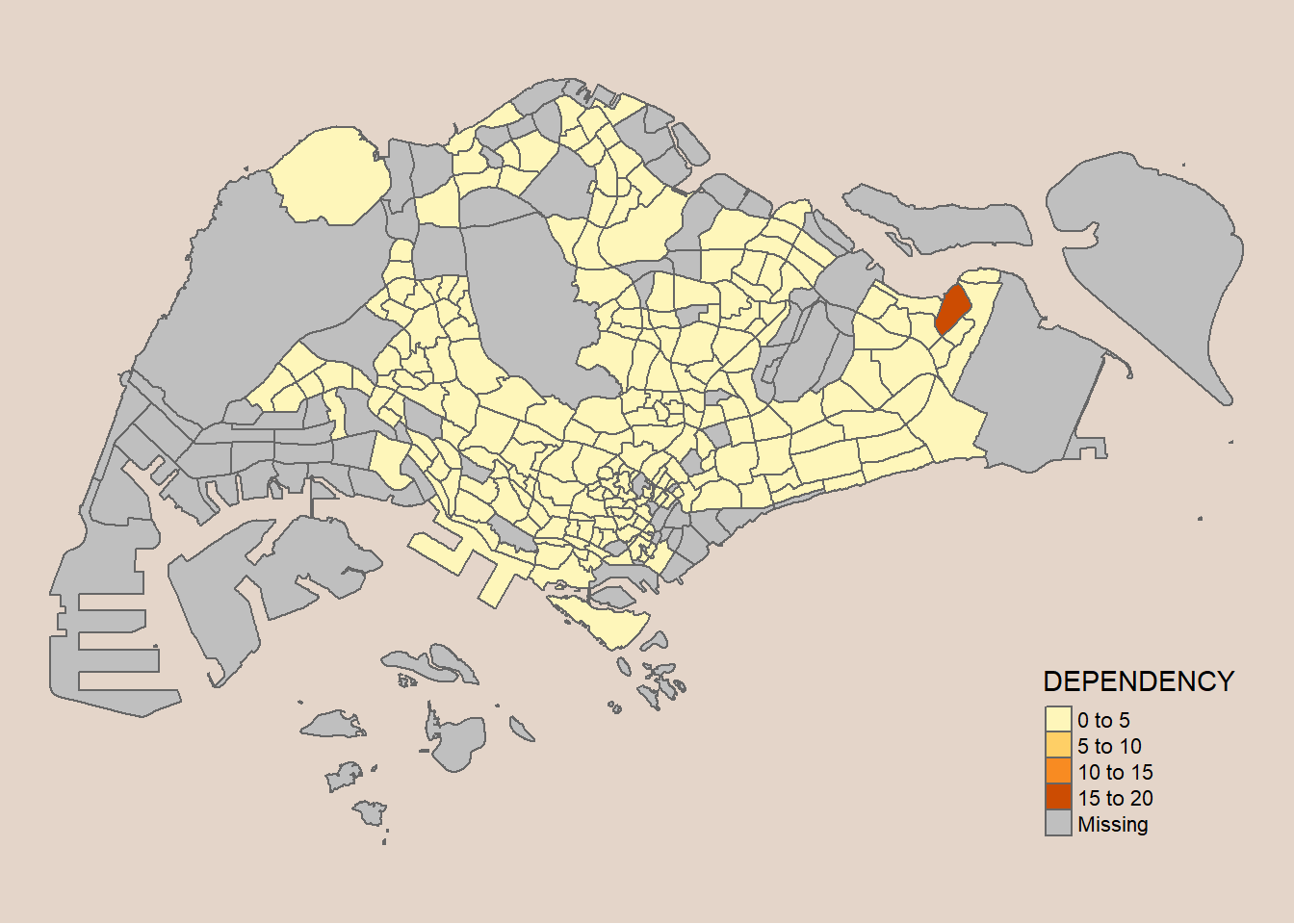
Things to learn from tm_polygons()
- The default interval binning used to draw the choropleth map is called
pretty. - The default colour scheme used is
YlOrRdof ColorBrewer. - By default, missing value will be shaded in grey.
5.2.3 Drawing a choropleth map using tm_fill() and tm_border()
tm_polygons()is a wraper oftm_fill()andtm_border().tm_fill()shades the polygons by using the default colour schemetm_borders()adds the borders of the shapefile onto the choropleth map.
The code chunk below draws a choropleth map by using tm_fill() alone.
tm_shape(mpsz_pop2020)+
  tm_fill("DEPENDENCY") +
  tm_layout(bg.color = "#E4D5C9",
            frame = F)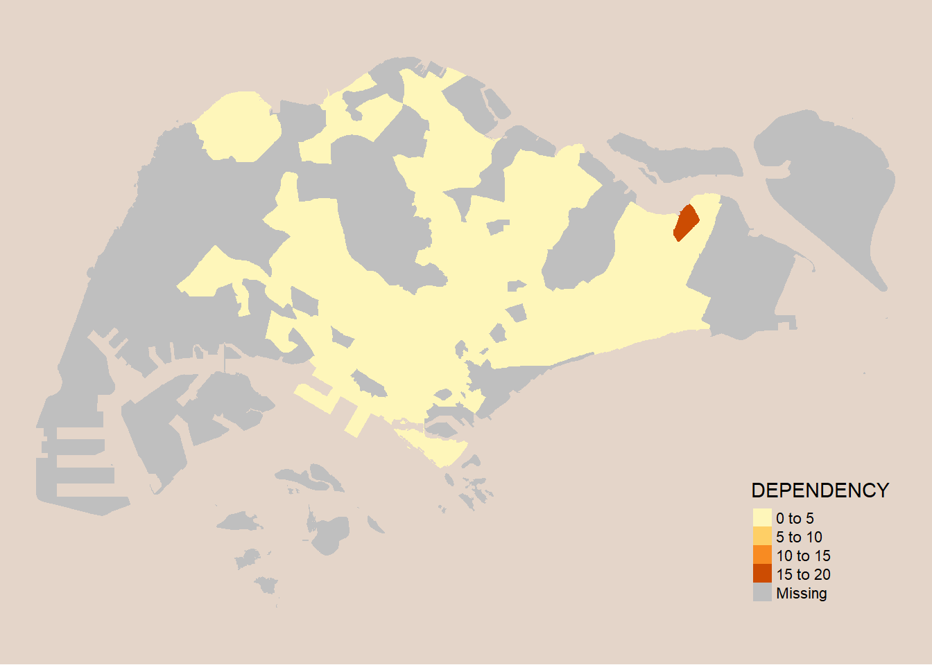
Notice that the planning subzones are shared according to the respective dependency values. To add the boundary of the planning subzones, tm_borders() will be used as shown in the code chunk below.
tm_shape(mpsz_pop2020)+
  tm_fill("DEPENDENCY") +
  tm_borders(lwd = 0.8,  alpha = 0.3) +
  tm_layout(bg.color = "#E4D5C9",
            frame = F)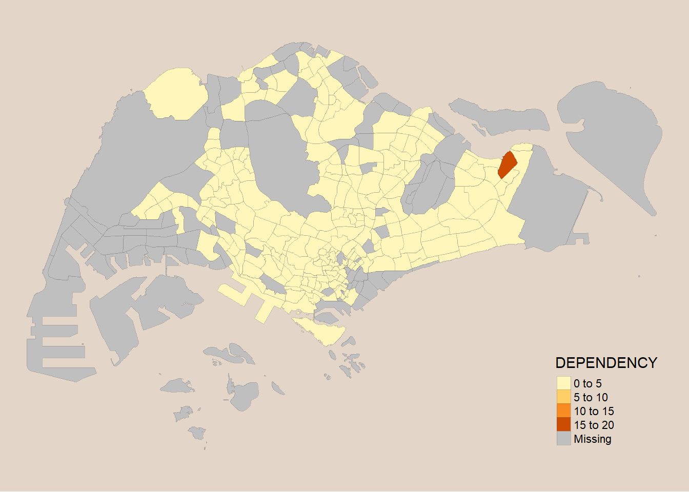
Light-gray border lines have been added on the choropleth map.
alpha argument: used to define transparency number between 0 (totally transparent) and 1 (not transparent). Default = 1.
col: border colour
lwd: border line width. Default = 1.
lty: border line type. Default = “solid”
5.3 Data classification methods of tmap
Most choropleth maps employ some methods of data classification. The point of classification is to take a large number of observations and group them into data ranges or classes.
tmap provides a total ten data classification methods, namely: fixed, sd, equal, pretty (default), quantile, kmeans, hclust, bclust, fisher, and jenks. To define a data classification method, the style argument of tm_fill() or tm_polygons() will be used.
5.3.1 Plotting choropleth maps with built-in classification methods
The code chunk below shows a quantile data classification that used 5 classes.
tm_shape(mpsz_pop2020)+
  tm_fill("DEPENDENCY",
          n = 5,
          style = "quantile") +
  tm_borders(alpha = 0.5) +
  tm_layout(bg.color = "#E4D5C9",
            frame = F)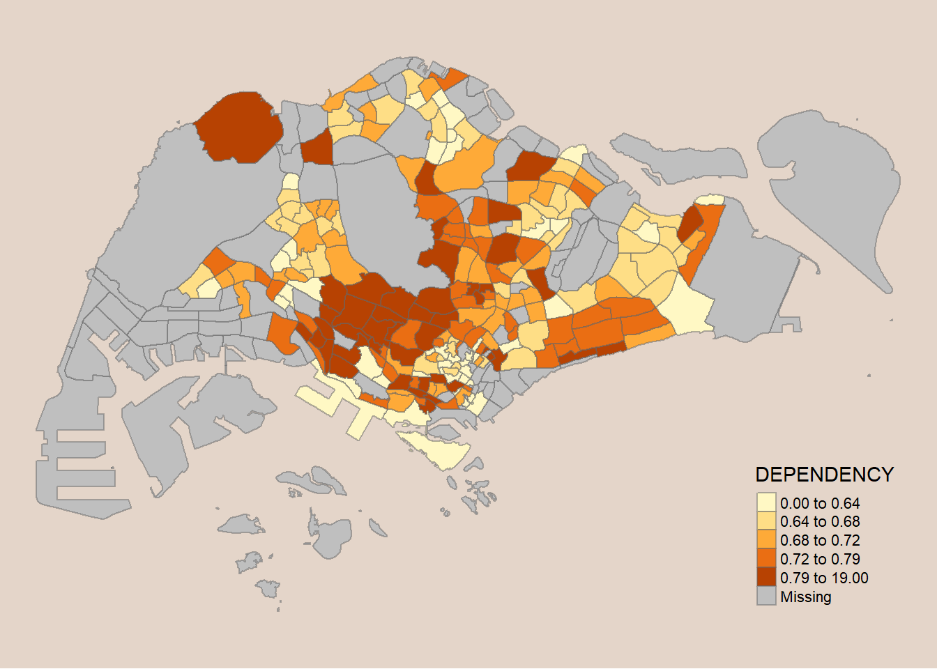
tm_shape(mpsz_pop2020)+
  tm_fill("DEPENDENCY",
          n = 5,
          style = "jenks") +
  tm_borders(alpha = 0.5) +
  tm_layout(bg.color = "#E4D5C9",
            frame = F)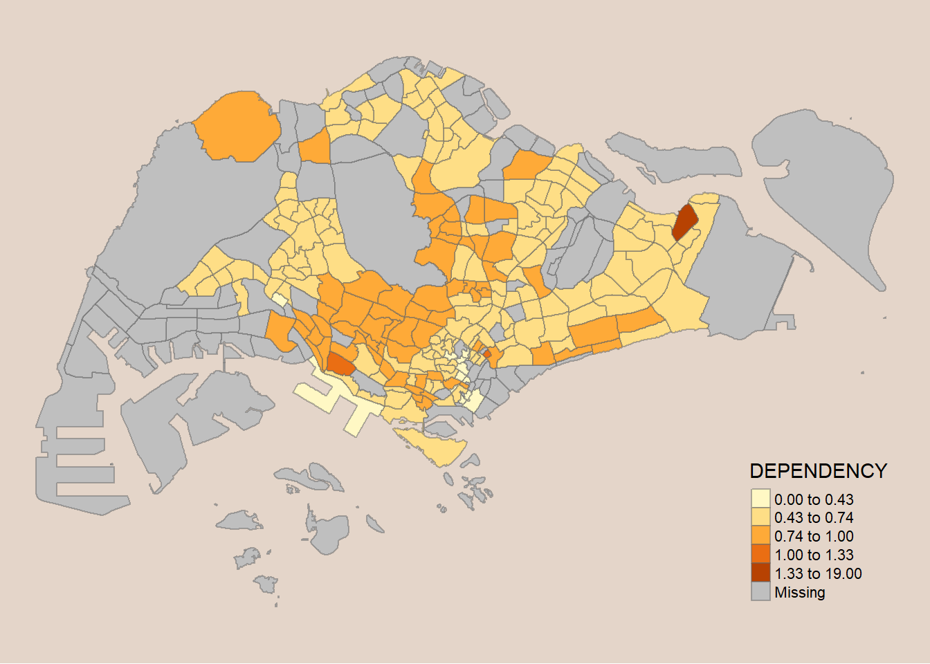
tm_shape(mpsz_pop2020)+
  tm_fill("DEPENDENCY",
          n = 5,
          style = "equal") +
  tm_borders(alpha = 0.5) +
  tm_layout(bg.color = "#E4D5C9",
            frame = F)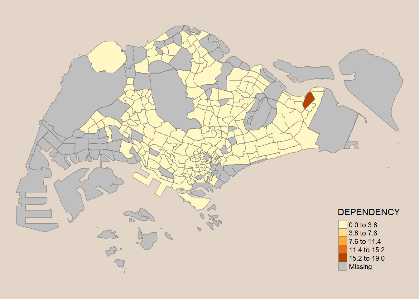
Notice that the distribution of quantile data classification method are more evenly distributed then equal data classification method.
tm_shape(mpsz_pop2020)+
  tm_fill("DEPENDENCY",
          n = 5,
          style = "sd") +
  tm_borders(alpha = 0.5) +
  tm_layout(bg.color = "#E4D5C9",
            frame = F)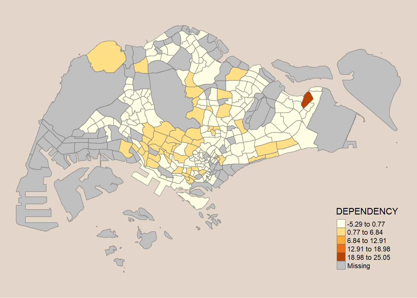
tm_shape(mpsz_pop2020)+
  tm_fill("DEPENDENCY",
          n = 2,
          style = "jenks") +
  tm_borders(alpha = 0.5)+
  tm_layout(bg.color = "#E4D5C9",
            frame = F)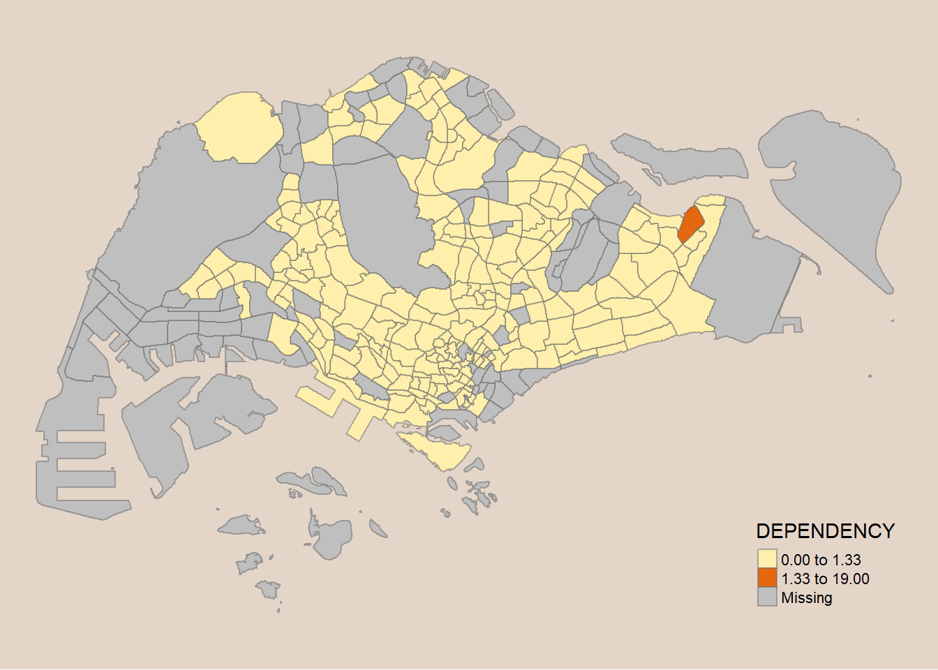
tm_shape(mpsz_pop2020)+
  tm_fill("DEPENDENCY",
          n = 5,
          style = "jenks") +
  tm_borders(alpha = 0.5) +
  tm_layout(bg.color = "#E4D5C9",
            frame = F)
tm_shape(mpsz_pop2020)+
  tm_fill("DEPENDENCY",
          n = 6,
          style = "jenks") +
  tm_borders(alpha = 0.5) +
  tm_layout(bg.color = "#E4D5C9",
            frame = F)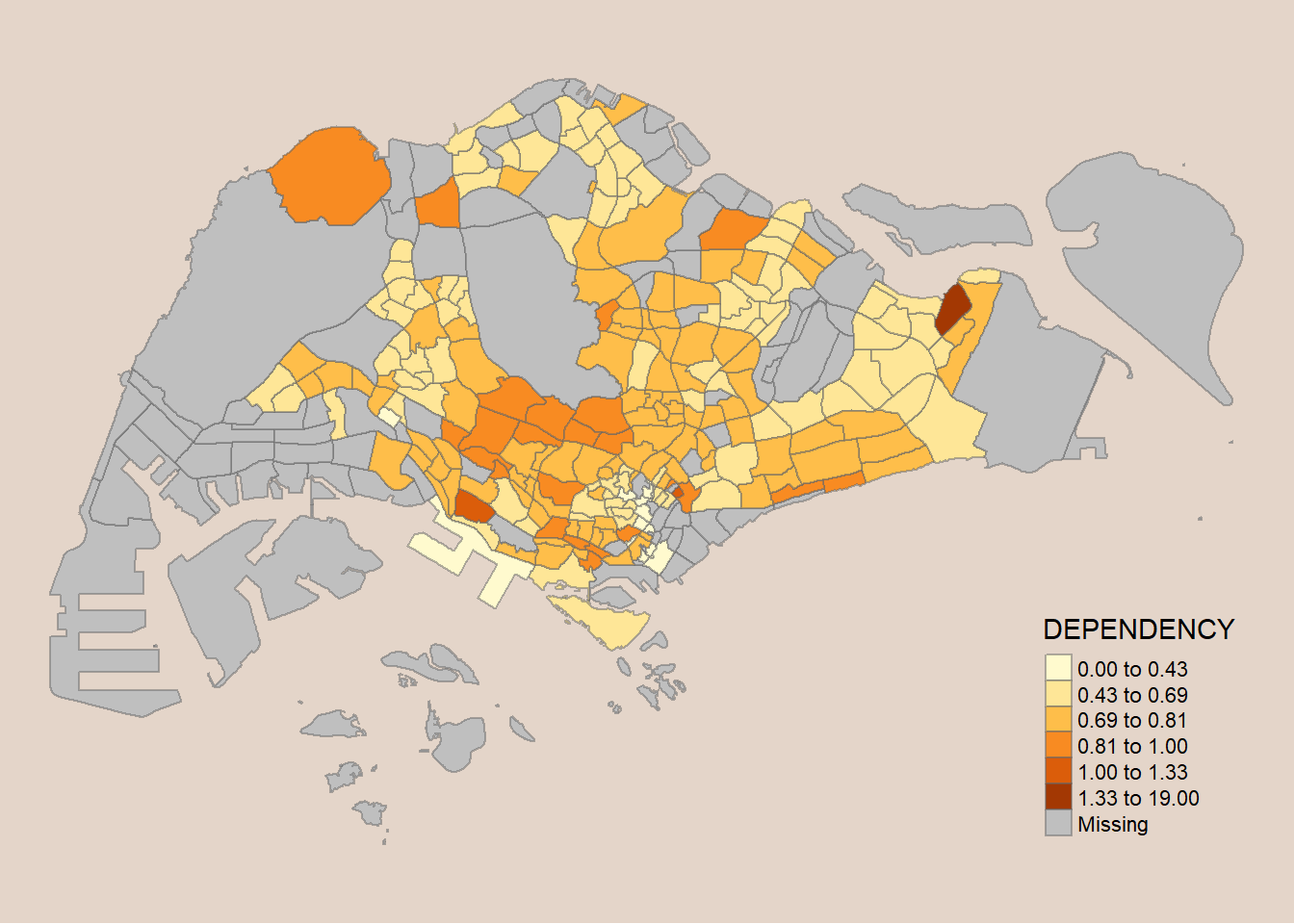
tm_shape(mpsz_pop2020)+
  tm_fill("DEPENDENCY",
          n = 10,
          style = "jenks") +
  tm_borders(alpha = 0.5)+
  tm_layout(bg.color = "#E4D5C9",
            frame = F)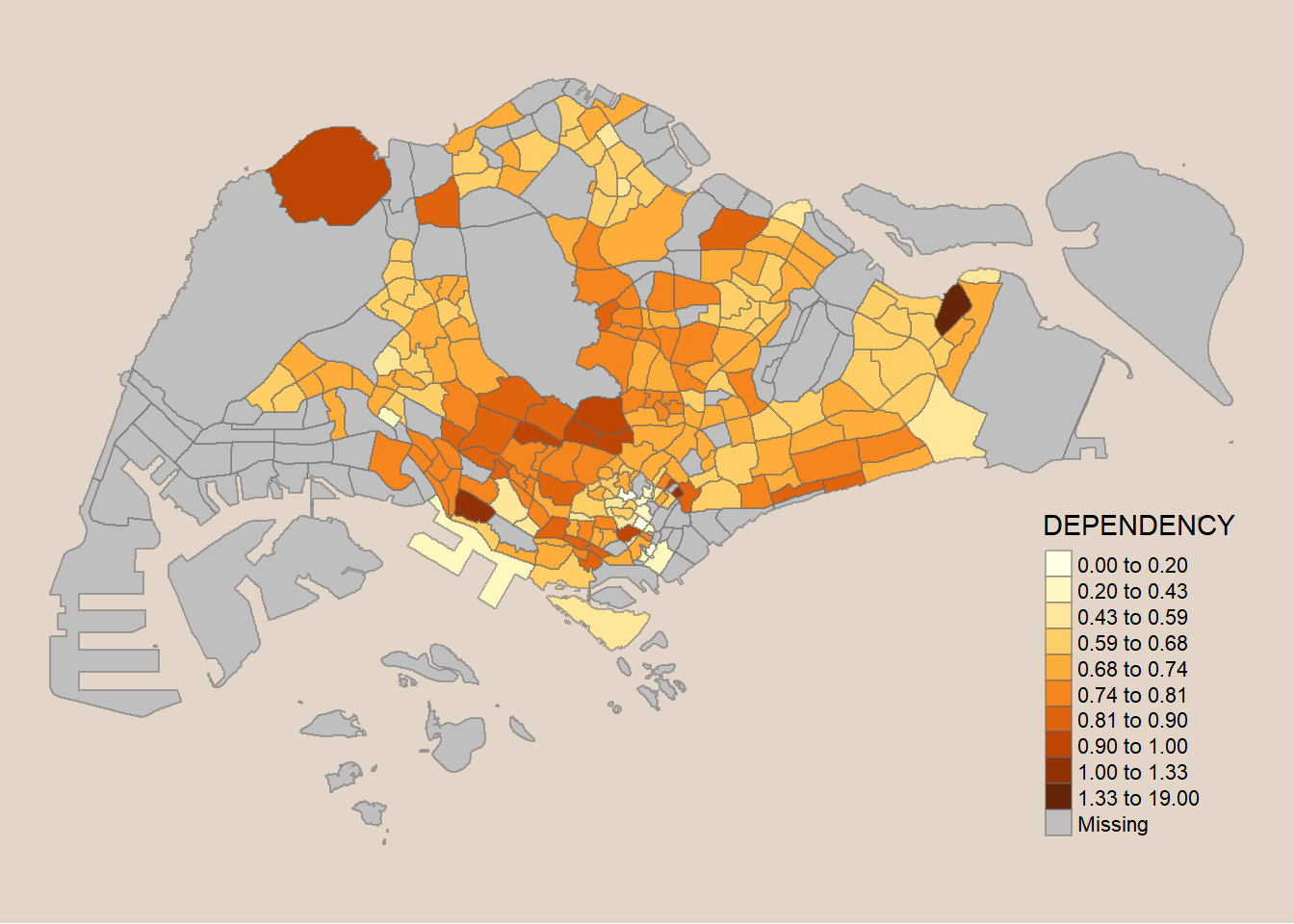
5.3.2 Plotting choropleth map with custom break
For all the built-in styles, the category breaks are computed internally. In order to override these defaults, the breakpoints can be set explicitly by means of the breaks argument to the tm_fill().
It is important to note that, in tmap the breaks include a minimum and maximum. As a result, in order to end up with n categories, n+1 elements must be specified in the breaks option (the values must be in increasing order).
Before we get started, it is always a good practice to get some descriptive statistics on the variable before setting the break points. Code chunk below will be used to compute and display the descriptive statistics of DEPENDENCY field.
summary(mpsz_pop2020$DEPENDENCY) Min. 1st Qu. Median Mean 3rd Qu. Max. NA's
0.0000 0.6519 0.7025 0.7742 0.7645 19.0000 92 With reference to the results above, we set break point at 0.60, 0.70, 0.80, and 0.90. In addition, we also need to include a minimum and maximum, which we set at 0 and 100. Our breaks vector is thus c(0, 0.60, 0.70, 0.80, 0.90, 1.00).
Now, we will plot the choropleth map by using the code chunk below.
tm_shape(mpsz_pop2020)+
  tm_fill("DEPENDENCY",
          breaks = c(0, 0.60, 0.70, 0.80, 0.90, 1.00)) +
  tm_borders(alpha = 0.5) +
  tm_layout(bg.color = "#E4D5C9",
            frame = F)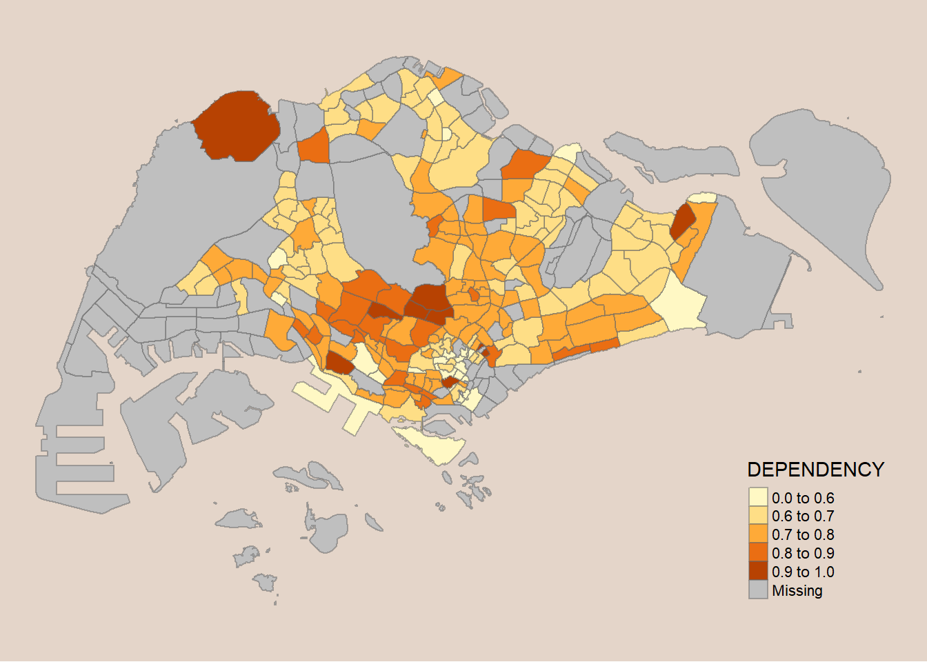
5.4 Colour Scheme
tmap supports colour ramps either defined by the user or a set of predefined colour ramps from the RColorBrewer package.
To change the colour, we assign the preferred colour to palette argument of tm_fill() as shown in the code chunk below.
tm_shape(mpsz_pop2020)+
  tm_fill("DEPENDENCY",
          n = 6,
          style = "quantile",
          palette = "Blues") +
  tm_borders(alpha = 0.5) +
  tm_layout(bg.color = "#E4D5C9",
            frame = F)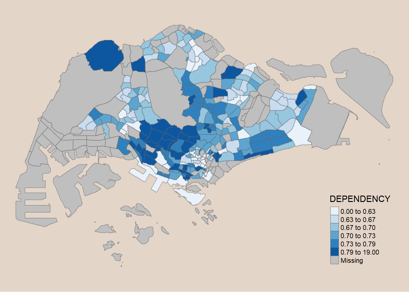
tm_shape(mpsz_pop2020)+
  tm_fill("DEPENDENCY",
          style = "quantile",
          palette = "Spectral") +
  tm_borders(alpha = 0.5) +
  tm_layout(bg.color = "#E4D5C9",
            frame = F)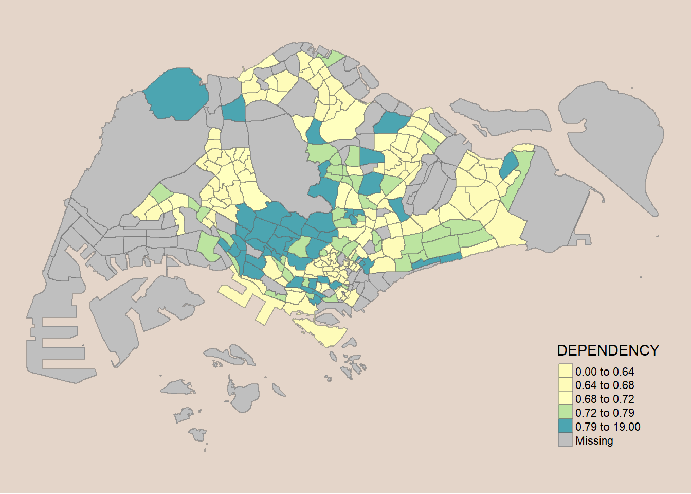
Notice that the choropleth map is shaded in green. To reverse the colour shading, add a - prefix.
tm_shape(mpsz_pop2020)+
  tm_fill("DEPENDENCY",
          style = "quantile",
          palette = "-Greens") +
  tm_borders(alpha = 0.5) +
  tm_layout(bg.color = "#E4D5C9",
            frame = F)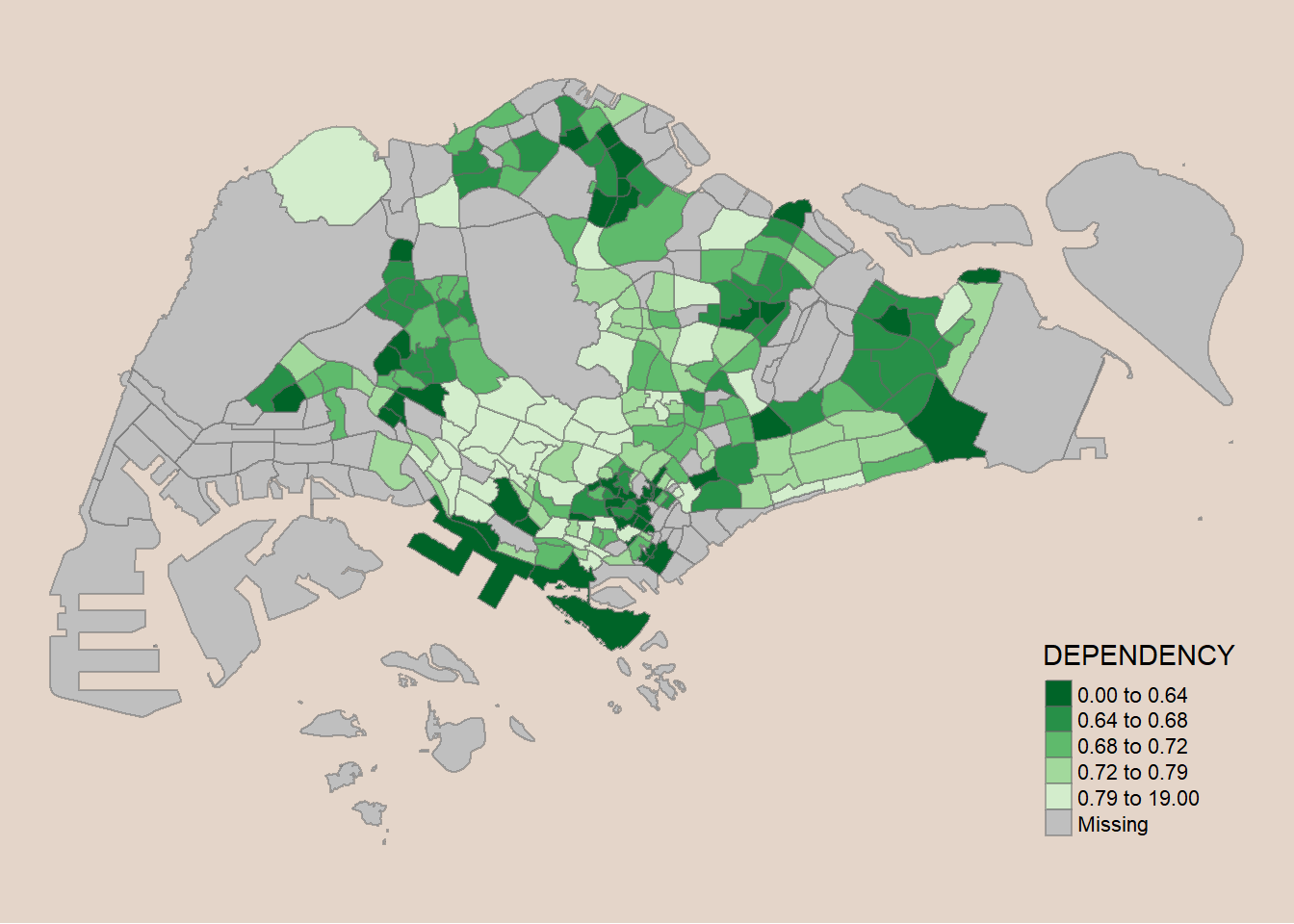
mine <- c('#c2c4b6','#f7f0c6','#dadada','#abb6c8', '#5D7599')tm_shape(mpsz_pop2020)+
tm_fill("DEPENDENCY",
style = "quantile",
palette = mine) +
tm_borders(alpha = 0.5) +
tm_layout(bg.color = "#E4D5C9",
frame = F)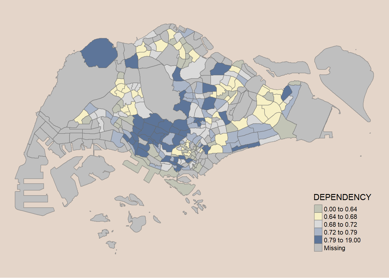
5.5 Map Layouts
Map layout refers to the combination of all map elements into a cohesive map. Map elements include among others the objects to be mapped, the title, the scale bar, the compass, margins and aspects ratios.
Colour settings and data classification methods covered in the previous section relate to the palette and break-points are used to affect how the map looks.
5.5.1 Map Legend
In tmap, several legend options are provided to change the placement, format and appearance of the legend.
tm_shape(mpsz_pop2020)+

  tm_fill("DEPENDENCY",
          style = "jenks",
          palette = "Blues",
          legend.hist = TRUE,
          legend.is.portrait = TRUE,
          legend.hist.z = 0.1) +

  tm_layout(main.title = "Distribution of Dependency Ratio by planning subzone \n(Jenks classification)",
            main.title.position = "center",
            main.title.size = 1,
            legend.height = 0.42,
            legend.width = 0.35,
            legend.outside = FALSE,
            legend.position = c("right", "bottom"),
            frame = FALSE,
            bg.color = "#E4D5C9") +

  tm_borders(alpha = 0.5)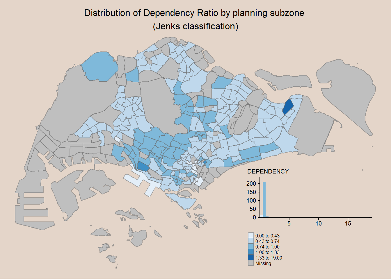
5.5.2 Map style
tmap allows a wide variety of layout settings to be changed. They can be called by using tmap_style(). The code chunk below shows the classic style is used.
tm_shape(mpsz_pop2020)+
  tm_fill("DEPENDENCY",
          style = "quantile",
          palette = "-Greens") +
  tm_borders(alpha = 0.5) +
  tmap_style("classic") +
  tm_layout(bg.color = "#E4D5C9",
            frame = T)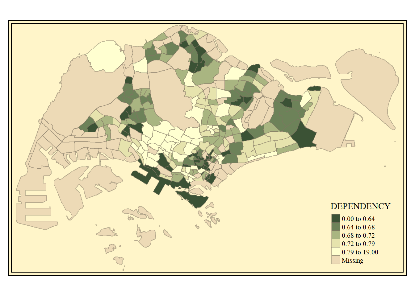
5.5.3 Cartographic Furniture
tmap also also provides arguments to draw other map furniture such as compass, scale bar and grid lines.
To reset the default style, use code chunk below:
tmap_style("white")In the code chunk below, tm_compass(), tm_scale_bar() and tm_grid() are used to add compass, scale bar and grid lines onto the choropleth map.
tm_shape(mpsz_pop2020)+
  tm_fill("DEPENDENCY",
          style = "quantile",
          palette = "Blues",
          title = "No. of persons") +
  tm_layout(main.title = "Distribution of Dependency Ratio \nby planning subzone",
            main.title.position = "center",
            main.title.size = 1.0,
            legend.height = 0.45,
            legend.width = 0.35,
            frame = F,
            bg.color = "#E4D5C9") +
  tm_borders(alpha = 0.5) +
  tm_compass(size = 1.8) +
  tm_scale_bar(width = 0.1) +
  tm_grid(lwd = 0.1, alpha = 0.2) +
  tm_credits("Source: Planning Sub-zone boundary from Urban Redevelopment Authorithy (URA)\n and Population data from Department of Statistics DOS",
             position = c("left", "bottom"))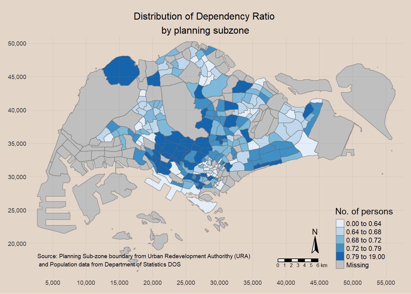
5.5.4 Drawing Small Multiple Choropleth Maps
Small multiple maps aka facet maps, are composed of many maps arrange side-by-side, and sometimes stacked vertically.
Small multiple maps enable the visualisation of how spatial relationships change with respect to another variable, such as time.
In tmap, small multiple maps can be plotted in three ways:
- by assigning multiple values to at least one of the asthetic arguments,
- by defining a group-by variable in
tm_facets(), and - by creating multiple stand-alone maps with
tmap_arrange().
In this example, small multiple choropleth maps are created by defining ncols in tm_fill().
tm_shape(mpsz_pop2020)+
  tm_fill(c("YOUNG", "AGED"), #<< 2 items
          style = "equal",
          palette = "Blues") +
  tm_layout(legend.position = c("right", "bottom"),
            bg.color = "#E4D5C9",
            frame = F) +
  tm_borders(alpha = 0.5)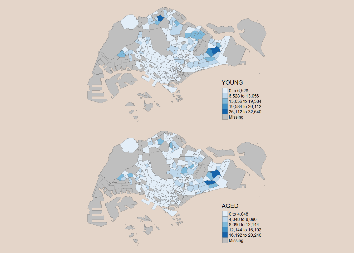
In this example, small multiple choropleth maps are created by assigning multiple values to at least one of the aesthetic arguments.
tm_shape(mpsz_pop2020)+
  tm_polygons(c("DEPENDENCY","AGED"),
          style = c("quantile", "quantile"),
          palette = list("Blues","Greens")) +
  tm_layout(main.title = "Distribution of Dependency Ratio vs Aged Population\n by Planning Subzone",
            main.title.position = "center",
            main.title.size = 0.8,
    legend.position = c("right", "bottom"),
            bg.color = "#E4D5C9",
            frame = F)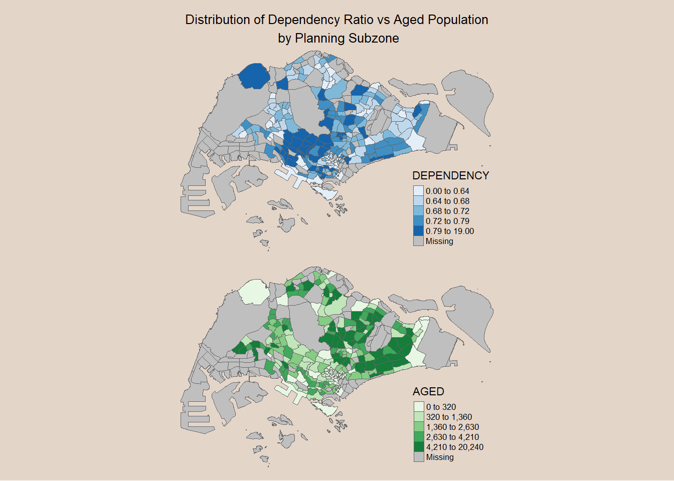
In this example, multiple small choropleth maps are created by using tm_facets().
Splits maps into groups ie by region
tm_shape(mpsz_pop2020) +
  tm_fill("DEPENDENCY",
          style = "quantile",
          palette = "Blues",
          thres.poly = 0) +

  tm_facets(by="REGION_N",  #<< Breakdown by Region
            free.coords=TRUE,
            drop.shapes=TRUE) +
  tm_layout(legend.show = FALSE,
            title.position = c("center", "center"),
            title.size = 20,
            bg.color = "#E4D5C9",
            frame = F) +
  tm_borders(alpha = 0.5)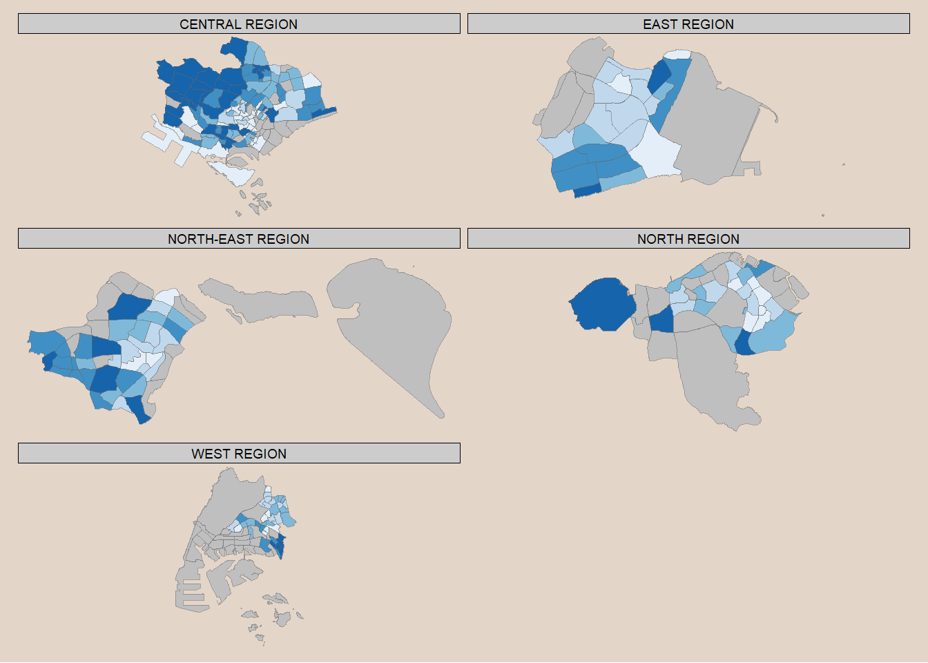
- In this example, multiple small choropleth maps are created by creating multiple stand-alone maps with
tmap_arrange().
youngmap <- tm_shape(mpsz_pop2020)+
  tm_polygons("YOUNG",
              style = "quantile",
              palette = "Blues") +
  tm_layout(bg.color = "#E4D5C9",
            frame = F)

agedmap <- tm_shape(mpsz_pop2020)+
  tm_polygons("AGED",
              style = "quantile",
              palette = "Blues") +
  tm_layout(bg.color = "#E4D5C9",
            frame = F)

tmap_arrange(youngmap, agedmap, asp=1, ncol=2)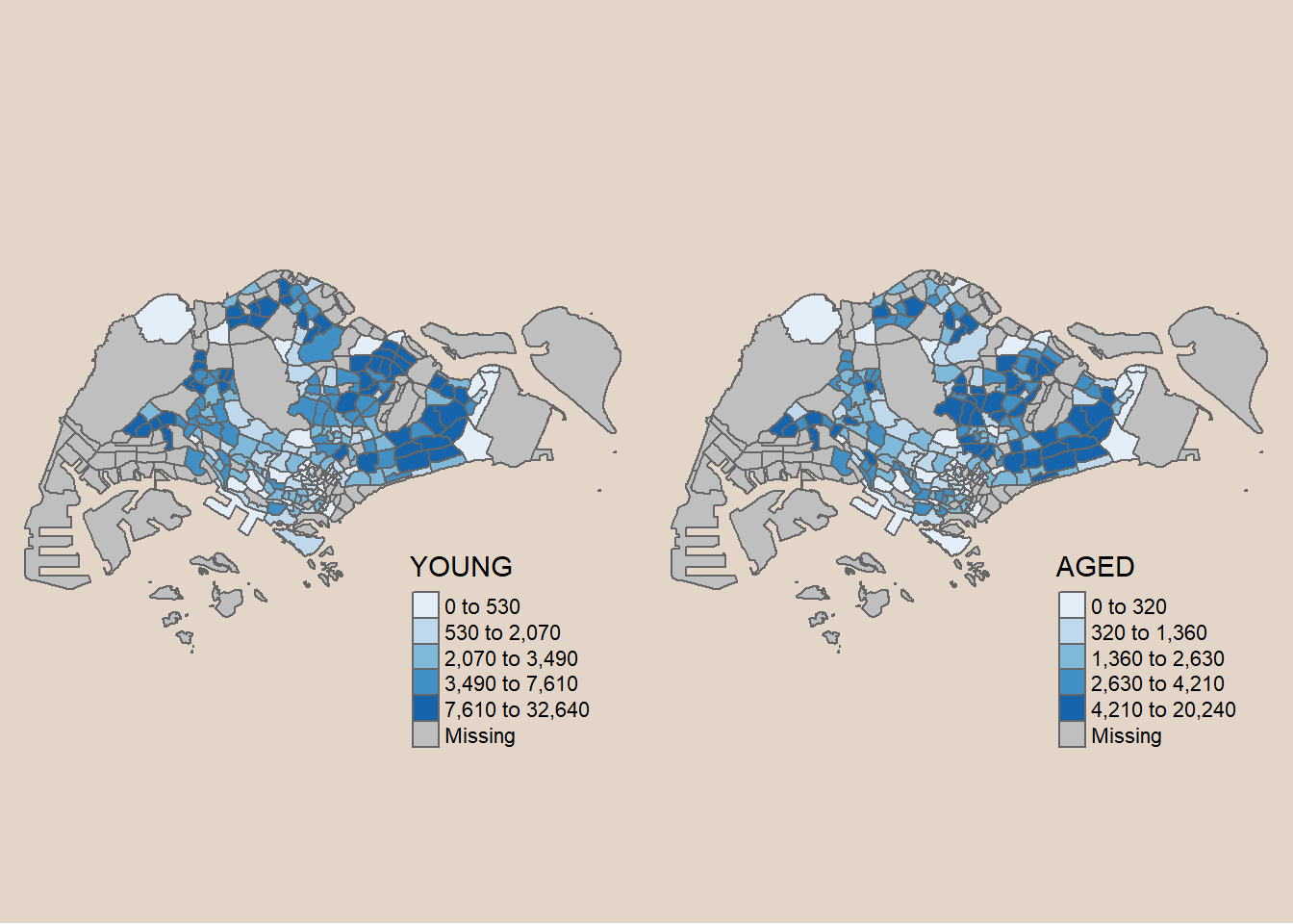
5.5.5 Mappping Spatial Object Meeting a Selection Criterion
Instead of creating small multiple choropleth map, you can also use selection funtion to map spatial objects meeting the selection criterion.
Below code only displays portion of the map where Region = Central Region.
tm_shape(mpsz_pop2020[mpsz_pop2020$REGION_N=="CENTRAL REGION", ])+ #<< == Central
  tm_fill("DEPENDENCY",
          style = "quantile",
          palette = "Blues",
          legend.hist = TRUE,
          legend.is.portrait = TRUE,
          legend.hist.z = 0.1) +
  tm_layout(legend.outside = TRUE,
            legend.height = 0.45,
            legend.width = 5.0,
            legend.position = c("right", "bottom"),
            bg.color = "#E4D5C9",
            frame = F) +
  tm_borders(alpha = 0.5)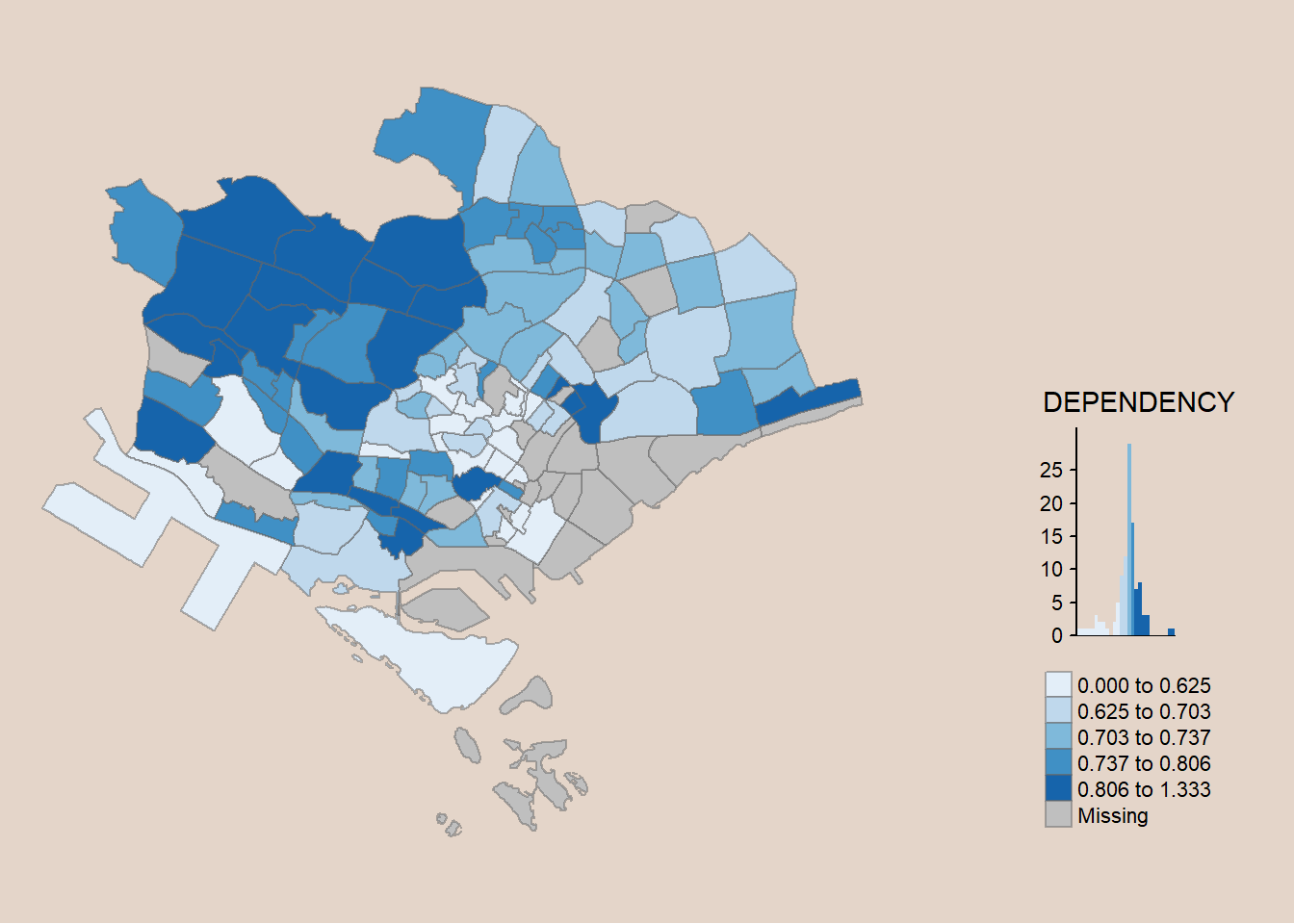
6 Reference
Kam, T. S. Thematic Mapping and Geovisualisation with R. R for Geospatial Data Science and Analytics. https://r4gdsa.netlify.app/chap02.html