pacman::p_load(sf, tmap,
stplanr,
performance,
ggpubr,
tidyverse,
DT, knitr, kableExtra)1 Overview
Spatial interaction represent the flow of people, material, or information between locations in geographical space. It encompasses everything from freight shipments, energy flows, and the global trade in rare antiquities, to flight schedules, rush hour woes, and pedestrian foot traffic.
Each spatial interaction, as an analogy for a set of movements, is composed of a discrete origin/destination pair. Each pair can be represented as a cell in a matrix where rows are related to the locations (centroids) of origin, while columns are related to locations (centroids) of destination. Such a matrix is commonly known as an origin/destination matrix, or a spatial interaction matrix.
Conditions for Spatial Flows
Three interdependent conditions are necessary for a spatial interaction to occur:
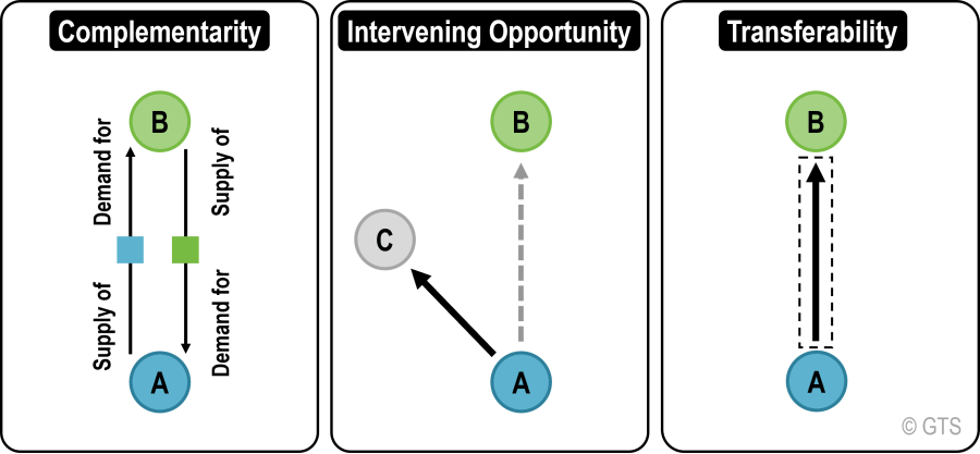
Features
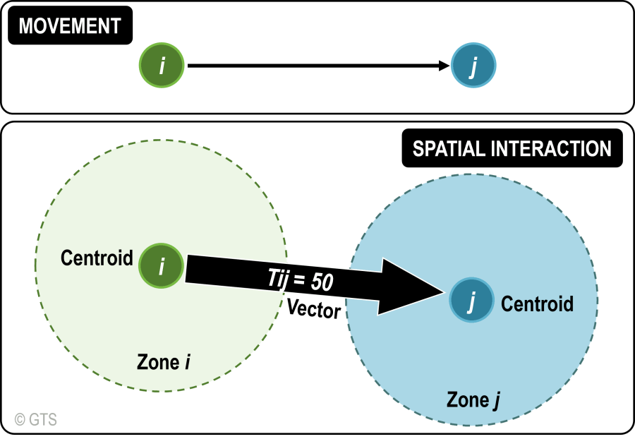
- Locations: A movement is occurring between a location of origin and a location of destination (\(i\) = origin; \(j\) = destination)
- Centroid: Abstraction of the attributes of a zone at a point
- Flows: Expressed by a valued vector \(T_{ij}\) representing an interaction between locations \(i\) and \(j\)
- Vectors: A vector \(T_{ij}\) links two centroids and has a value assigned to it (50) which can represents movements
Task
In this hands-on exercise, we will learn how to build an OD matrix by using Passenger Volume by Origin Destination Bus Stops data set downloaded from LTA DataMall. By the end of this hands-on exercise, we will be able:
- to import and extract OD data for a selected time interval,
- to import and save geospatial data (i.e. bus stops and mpsz) into sf tibble data frame objects,
- to populate planning subzone code into bus stops sf tibble data frame,
- to construct desire lines geospatial data from the OD data, and
- to visualise passenger volume by origin and destination bus stops by using the desire lines data.
2 The Packages
| Package | Usage |
|---|---|
| sf | For importing, integrating, processing and transforming geospatial data |
| tmap | Choropleth mapping; thematic maps |
| stplanr | For sustainable transport planning; provides functions and tools for analysis and visualisation of transport projects |
| performance | For model performance measurement |
| ggpubr | For visualisation |
| tidyverse | For importing, integrating, wrangling and visualising data |
| DT, knitr, kableExtra | For building tables |
3 The Data
3.1 Aspatial
| Step | Description | Screenshot |
|---|---|---|
| 1. | Under Dynamic Datasets of the LTA DataMall, click on ‘Request API Access’. Fill up the request accordingly. | |
| 2. | Follow instructions from LTA DataMall API User Guide to download and install Postman. Launch Postman app once completed. | |
| 2. | From LTA DataMall API User Guide & Documentation, search for Passenger Volume by Origin Destination Bus Stops. Copy the URL indicated in the table. | |
| 3. | In the Postman app, paste URL copied in the field beside ‘GET’. Under ‘Params’ tab, enter the following details:
|
|
| 4. | Under ‘Headers’, enter the following details:
Click ‘Send’. |
|
| 5. | A URL will be generated. Press Ctrl + Click to download the dataset. This will be in a .zip file format. |
3.2 Geospatial
Two geospatial data will be used. They are:
| Name | Details | Screenshot |
|---|---|---|
| BusStop, from LTA DataMall > Static Datasets |
|
|
| MPSZ-2019 |
|
4 Preparing Flow Data
4.1 Importing OD data
odbus <- read_csv("data/aspatial/origin_destination_bus_202407.csv")glimpse(odbus)Rows: 5,476,662
Columns: 7
$ YEAR_MONTH <chr> "2024-07", "2024-07", "2024-07", "2024-07", "2024-…
$ DAY_TYPE <chr> "WEEKENDS/HOLIDAY", "WEEKDAY", "WEEKDAY", "WEEKEND…
$ TIME_PER_HOUR <dbl> 16, 16, 14, 14, 17, 17, 17, 7, 17, 14, 14, 10, 20,…
$ PT_TYPE <chr> "BUS", "BUS", "BUS", "BUS", "BUS", "BUS", "BUS", "…
$ ORIGIN_PT_CODE <chr> "04168", "04168", "80119", "80119", "44069", "4406…
$ DESTINATION_PT_CODE <chr> "10051", "10051", "90079", "90079", "17229", "1722…
$ TOTAL_TRIPS <dbl> 5, 4, 3, 1, 1, 1, 14, 3, 2, 2, 1, 4, 5, 1, 1, 4, 1…odbus tibble data frame shows that the values in ORIGIN_PT_CODE and DESTINATON_PT_CODE are in numeric data type. Hence, the code chunk below is used to convert these data values into character data type.
odbus$ORIGIN_PT_CODE <- as.factor(odbus$ORIGIN_PT_CODE)
odbus$DESTINATION_PT_CODE <- as.factor(odbus$DESTINATION_PT_CODE) Recheck to confirm that the 2 variables have indeed been updated:
glimpse(odbus)Rows: 5,476,662
Columns: 7
$ YEAR_MONTH <chr> "2024-07", "2024-07", "2024-07", "2024-07", "2024-…
$ DAY_TYPE <chr> "WEEKENDS/HOLIDAY", "WEEKDAY", "WEEKDAY", "WEEKEND…
$ TIME_PER_HOUR <dbl> 16, 16, 14, 14, 17, 17, 17, 7, 17, 14, 14, 10, 20,…
$ PT_TYPE <chr> "BUS", "BUS", "BUS", "BUS", "BUS", "BUS", "BUS", "…
$ ORIGIN_PT_CODE <fct> 04168, 04168, 80119, 80119, 44069, 44069, 20281, 1…
$ DESTINATION_PT_CODE <fct> 10051, 10051, 90079, 90079, 17229, 17229, 20141, 1…
$ TOTAL_TRIPS <dbl> 5, 4, 3, 1, 1, 1, 14, 3, 2, 2, 1, 4, 5, 1, 1, 4, 1…4.2 Extracting study data
For our study, we will extract commuting flows on weekday and between 6 and 9 o’clock.
odbus6_9 <- odbus %>%
filter(DAY_TYPE == "WEEKDAY") %>%
filter(TIME_PER_HOUR >= 6 &
TIME_PER_HOUR <= 9) %>%
group_by(ORIGIN_PT_CODE,
DESTINATION_PT_CODE) %>%
summarise(TRIPS = sum(TOTAL_TRIPS))We can use the datatable package for interactive tables:
Show the code
datatable(
odbus6_9,
filter='top')We will save the output in rds format for future use, and reimport the saved rds file into R environment:
write_rds(odbus6_9, "data/rds/odbus6_9.rds")
odbus6_9 <- read_rds("data/rds/odbus6_9.rds")5 Working with Geospatial Data
5.1 Importing geospatial data
5.1.1 Polygon data
st_read()function of sf package is used to import the shapefile into R as sf data frame.st_transform()function of sf package is used to transform the projection to crs 3414.
mpsz <- st_read(dsn = "data/geospatial",
layer = "MPSZ-2019") %>%
st_transform(crs = 3414)Reading layer `MPSZ-2019' from data source
`C:\kytjy\ISSS626-GAA\Hands-on_Ex\Hands-on_Ex09\data\geospatial'
using driver `ESRI Shapefile'
Simple feature collection with 332 features and 6 fields
Geometry type: MULTIPOLYGON
Dimension: XY
Bounding box: xmin: 103.6057 ymin: 1.158699 xmax: 104.0885 ymax: 1.470775
Geodetic CRS: WGS 84mpszSimple feature collection with 332 features and 6 fields
Geometry type: MULTIPOLYGON
Dimension: XY
Bounding box: xmin: 2667.538 ymin: 15748.72 xmax: 56396.44 ymax: 50256.33
Projected CRS: SVY21 / Singapore TM
First 10 features:
SUBZONE_N SUBZONE_C PLN_AREA_N PLN_AREA_C REGION_N
1 MARINA EAST MESZ01 MARINA EAST ME CENTRAL REGION
2 INSTITUTION HILL RVSZ05 RIVER VALLEY RV CENTRAL REGION
3 ROBERTSON QUAY SRSZ01 SINGAPORE RIVER SR CENTRAL REGION
4 JURONG ISLAND AND BUKOM WISZ01 WESTERN ISLANDS WI WEST REGION
5 FORT CANNING MUSZ02 MUSEUM MU CENTRAL REGION
6 MARINA EAST (MP) MPSZ05 MARINE PARADE MP CENTRAL REGION
7 SUDONG WISZ03 WESTERN ISLANDS WI WEST REGION
8 SEMAKAU WISZ02 WESTERN ISLANDS WI WEST REGION
9 SOUTHERN GROUP SISZ02 SOUTHERN ISLANDS SI CENTRAL REGION
10 SENTOSA SISZ01 SOUTHERN ISLANDS SI CENTRAL REGION
REGION_C geometry
1 CR MULTIPOLYGON (((33222.98 29...
2 CR MULTIPOLYGON (((28481.45 30...
3 CR MULTIPOLYGON (((28087.34 30...
4 WR MULTIPOLYGON (((14557.7 304...
5 CR MULTIPOLYGON (((29542.53 31...
6 CR MULTIPOLYGON (((35279.55 30...
7 WR MULTIPOLYGON (((15772.59 21...
8 WR MULTIPOLYGON (((19843.41 21...
9 CR MULTIPOLYGON (((30870.53 22...
10 CR MULTIPOLYGON (((26879.04 26...summary(mpsz) SUBZONE_N SUBZONE_C PLN_AREA_N PLN_AREA_C
Length:332 Length:332 Length:332 Length:332
Class :character Class :character Class :character Class :character
Mode :character Mode :character Mode :character Mode :character
REGION_N REGION_C geometry
Length:332 Length:332 MULTIPOLYGON :332
Class :character Class :character epsg:3414 : 0
Mode :character Mode :character +proj=tmer...: 0 unique(mpsz$PLN_AREA_N) [1] "MARINA EAST" "RIVER VALLEY"
[3] "SINGAPORE RIVER" "WESTERN ISLANDS"
[5] "MUSEUM" "MARINE PARADE"
[7] "SOUTHERN ISLANDS" "BUKIT MERAH"
[9] "DOWNTOWN CORE" "STRAITS VIEW"
[11] "QUEENSTOWN" "OUTRAM"
[13] "MARINA SOUTH" "ROCHOR"
[15] "KALLANG" "TANGLIN"
[17] "NEWTON" "CLEMENTI"
[19] "BEDOK" "PIONEER"
[21] "JURONG EAST" "ORCHARD"
[23] "GEYLANG" "BOON LAY"
[25] "BUKIT TIMAH" "NOVENA"
[27] "TOA PAYOH" "TUAS"
[29] "JURONG WEST" "SERANGOON"
[31] "BISHAN" "TAMPINES"
[33] "BUKIT BATOK" "HOUGANG"
[35] "CHANGI BAY" "PAYA LEBAR"
[37] "ANG MO KIO" "PASIR RIS"
[39] "BUKIT PANJANG" "TENGAH"
[41] "SELETAR" "SUNGEI KADUT"
[43] "YISHUN" "MANDAI"
[45] "PUNGGOL" "CHOA CHU KANG"
[47] "SENGKANG" "CHANGI"
[49] "CENTRAL WATER CATCHMENT" "SEMBAWANG"
[51] "WESTERN WATER CATCHMENT" "WOODLANDS"
[53] "NORTH-EASTERN ISLANDS" "SIMPANG"
[55] "LIM CHU KANG" unique(mpsz$REGION_N)[1] "CENTRAL REGION" "WEST REGION" "EAST REGION"
[4] "NORTH-EAST REGION" "NORTH REGION" par(bg = '#E4D5C9')
par(mar = c(0,0,0,0))
plot(st_geometry(mpsz))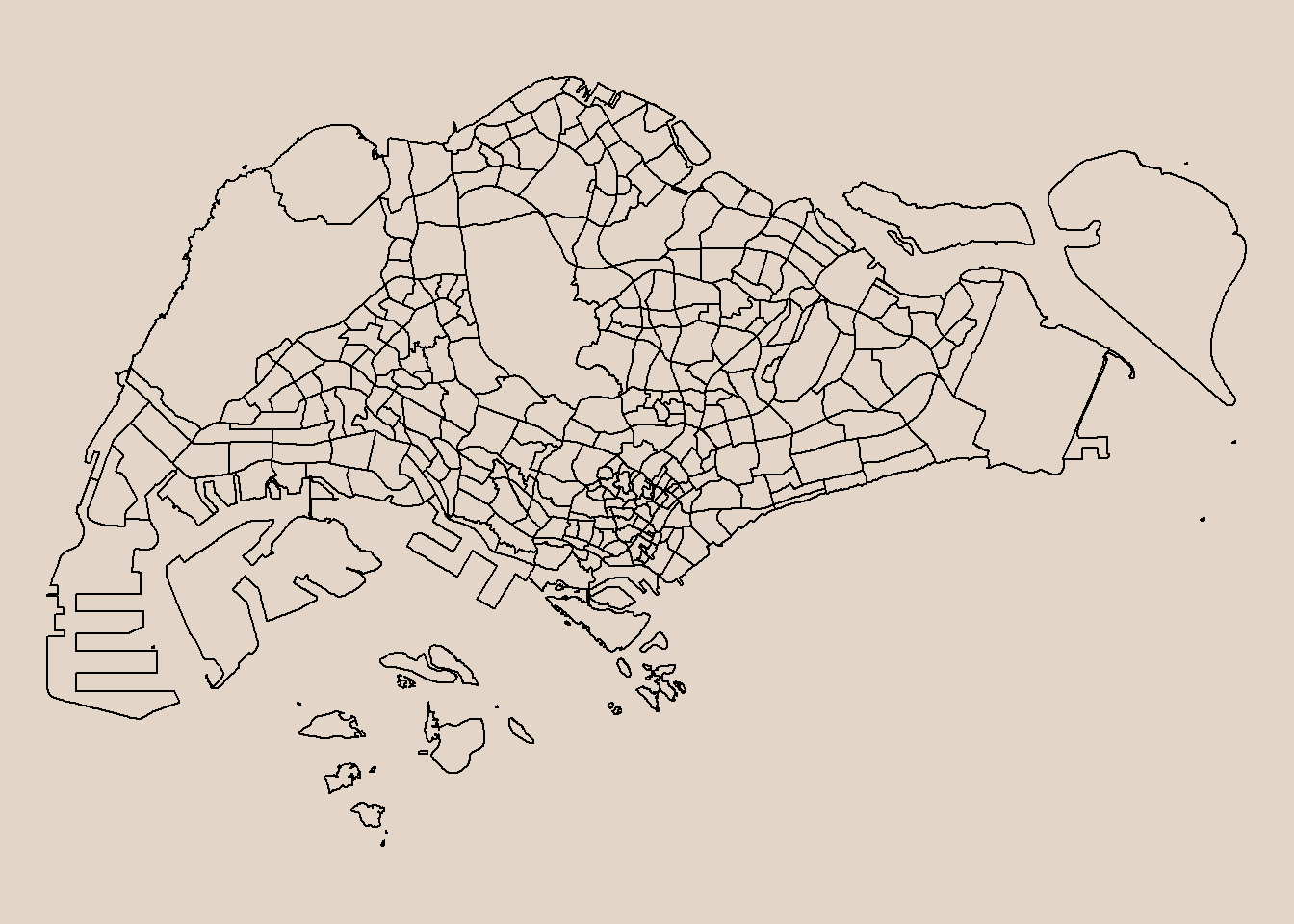
Observations
There are 332 subzones across 5 regions.
In the plot, we can also see that the MPSZ data includes outer islands of Singapore such as Sudong, Semakau, Southern Group, and North-Eastern islands. Since it’s unlikely to catch a bus to/from these islands, I’ll remove them from our data.
outerislands <- c("SEMAKAU", "SUDONG", "NORTH-EASTERN ISLANDS", "SOUTHERN GROUP")
# remove rows where 'SUBZONE_N' is in the list
mpsz <- mpsz %>%
filter(!str_trim(SUBZONE_N) %in% str_trim(outerislands))We’ll plot the mpsz again to ensure the outer islands have been removed.
par(bg = '#E4D5C9')
par(mar = c(0,0,0,0))
plot(st_geometry(mpsz))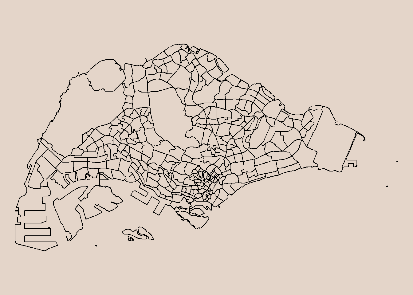
mpsz <- write_rds(mpsz, "data/rds/mpsz.rds")5.1.2 Point Data
busstop <- st_read(dsn = "data/geospatial",
layer = "BusStop") %>%
st_transform(crs = 3414)Reading layer `BusStop' from data source
`C:\kytjy\ISSS626-GAA\Hands-on_Ex\Hands-on_Ex09\data\geospatial'
using driver `ESRI Shapefile'
Simple feature collection with 5166 features and 3 fields
Geometry type: POINT
Dimension: XY
Bounding box: xmin: 3970.122 ymin: 26482.1 xmax: 48285.52 ymax: 52983.82
Projected CRS: SVY21duplicate <- busstop %>%
group_by(BUS_STOP_N) %>%
filter(n() > 1) %>%
ungroup()
duplicateSimple feature collection with 36 features and 3 fields
Geometry type: POINT
Dimension: XY
Bounding box: xmin: 13488.02 ymin: 31863.63 xmax: 44144.57 ymax: 47934
Projected CRS: SVY21 / Singapore TM
# A tibble: 36 × 4
BUS_STOP_N BUS_ROOF_N LOC_DESC geometry
<chr> <chr> <chr> <POINT [m]>
1 58031 UNK OPP CANBERRA DR (27111.07 47517.77)
2 47201 UNK <NA> (22616.75 47793.68)
3 58031 UNK OPP CANBERRA DR (27089.69 47570.9)
4 62251 B03 Bef Blk 471B (35500.54 39943.41)
5 22501 B02 Blk 662A (13489.09 35536.4)
6 82221 B01 BLK 3A (35323.6 33257.05)
7 68091 B01 AFT BAKER ST (32164.11 42695.98)
8 43709 B06 BLK 644 (18963.42 36762.8)
9 82221 B01 Blk 3A (35308.74 33335.17)
10 97079 B14 OPP ST. JOHN'S CRES (44055.75 38908.5)
# ℹ 26 more rowsObservations
There are duplicated bus stop numbers, but with different roof IDs and geometry. Some of them could be temporary bus stops within the month.
In the plot below, we can also see that some bus stop fall outside the Singapore administrative boundaries.
tm_shape(mpsz) +
tm_polygons(col = "#f5f5f5") +
tm_shape(busstop) +
tm_dots(col="#800200") +
tm_layout(bg.color = "#E4D5C9",
frame = F)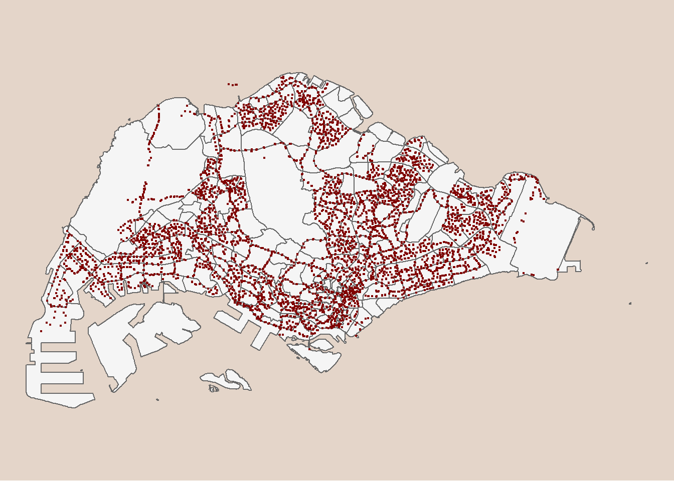
5.2 Geospatial data wrangling
5.2.1 Combine Busstop and mpsz
busstop_mpsz <- st_intersection(busstop, mpsz) %>%
select(BUS_STOP_N, SUBZONE_C) %>%
st_drop_geometry()Observations
Number of bus stop dropped from 5166 (busstop) to 5161 (busstop_mpsz) due to the 5 busstops outside MPSZ boundary (ie in Malaysia).
datatable(busstop_mpsz,
options = list(pageLength = 5))Save the output in rds format for future use:
write_rds(busstop_mpsz, "data/rds/busstop_mpsz.rds") 5.2.2 Append planning subzone code from busstop_mpsz onto odbus6_9
od_data <- left_join(odbus6_9 , busstop_mpsz,
by = c("ORIGIN_PT_CODE" = "BUS_STOP_N")) %>%
rename(ORIGIN_BS = ORIGIN_PT_CODE,
ORIGIN_SZ = SUBZONE_C,
DESTIN_BS = DESTINATION_PT_CODE)Observations
The number of records before the join is 238,490.
This increased to 239,372 after performing the left join.
5.2.3 Duplicates Check
Check for duplicates to prevent double counting:
duplicate2 <- od_data %>%
group_by_all() %>%
filter(n()>1) %>%
ungroup()
duplicate2# A tibble: 1,470 × 4
ORIGIN_BS DESTIN_BS TRIPS ORIGIN_SZ
<chr> <fct> <dbl> <chr>
1 09047 02029 2 ORSZ02
2 09047 02029 2 ORSZ02
3 09047 02049 54 ORSZ02
4 09047 02049 54 ORSZ02
5 09047 02089 35 ORSZ02
6 09047 02089 35 ORSZ02
7 09047 02151 98 ORSZ02
8 09047 02151 98 ORSZ02
9 09047 02161 35 ORSZ02
10 09047 02161 35 ORSZ02
# ℹ 1,460 more rowsIf duplicated records are found, the code chunk below will be used to retain the unique records.
od_data <- unique(od_data)Observations
There are 1,470 duplicated records in our data, i.e. 735 pairs.
Before removing duplicates: 239,372 After removal: 238,637
5.2.4 Update od_data with planning subzone codes
od_data <- left_join(od_data , busstop_mpsz,
by = c("DESTIN_BS" = "BUS_STOP_N")) Before: 238,637 After: 239,812
duplicate3 <- od_data %>%
group_by_all() %>%
filter(n()>1) %>%
ungroup()
duplicate3# A tibble: 1,844 × 5
ORIGIN_BS DESTIN_BS TRIPS ORIGIN_SZ SUBZONE_C
<chr> <chr> <dbl> <chr> <chr>
1 01013 51071 8 RCSZ10 CCSZ01
2 01013 51071 8 RCSZ10 CCSZ01
3 01112 51071 72 RCSZ10 CCSZ01
4 01112 51071 72 RCSZ10 CCSZ01
5 01112 53041 6 RCSZ10 BSSZ01
6 01112 53041 6 RCSZ10 BSSZ01
7 01113 51071 6 DTSZ01 CCSZ01
8 01113 51071 6 DTSZ01 CCSZ01
9 01113 82221 1 DTSZ01 GLSZ05
10 01113 82221 1 DTSZ01 GLSZ05
# ℹ 1,834 more rowsRetain unique records:
od_data <- unique(od_data)Before: 239,812 After: 238,890
5.2.5 Aggregate Data
od_data <- od_data %>%
# Rename column for better clarity
rename(DESTIN_SZ = SUBZONE_C) %>%
# Remove NAs (where there are missing subzones due to time diff between busstop & ridership info)
drop_na() %>%
# Group and summarise number of trips at each O/D level
group_by(ORIGIN_SZ, DESTIN_SZ) %>%
summarise(MORNING_PEAK = sum(TRIPS))
od_data# A tibble: 20,849 × 3
# Groups: ORIGIN_SZ [309]
ORIGIN_SZ DESTIN_SZ MORNING_PEAK
<chr> <chr> <dbl>
1 AMSZ01 AMSZ01 2435
2 AMSZ01 AMSZ02 10418
3 AMSZ01 AMSZ03 15578
4 AMSZ01 AMSZ04 2862
5 AMSZ01 AMSZ05 7938
6 AMSZ01 AMSZ06 2357
7 AMSZ01 AMSZ07 1513
8 AMSZ01 AMSZ08 2551
9 AMSZ01 AMSZ09 2358
10 AMSZ01 AMSZ10 291
# ℹ 20,839 more rowsBefore: 238,890 After: 20,849
Save the output in rds format for future use, and reimport into R environment:
write_rds(od_data, "data/rds/od_data.rds")
od_data <- read_rds("data/rds/od_data.rds")6 Visualising Spatial Interaction
In this section, we learn how to prepare a desired line by using stplanr package.
6.1 Remove intra-zonal flows
We will not plot the intra-zonal flows, i.e. where the origin and destination are the same (eg origin = AMSZ01 and destination = AMSZ01)
The code chunk below will be used to remove intra-zonal flows.
od_data1 <- od_data[od_data$ORIGIN_SZ!=od_data$DESTIN_SZ,]Before: 20,849 After: 20,558
The comma , after the condition is significant. In R’s data frame syntax, the format for subsetting is [rows, columns]. When you place a condition before the comma, it applies to rows. The comma itself then implies that you’re not applying any specific filter to the columns – meaning you want all columns.
6.2 Create desired lines
flowLine <- od2line(flow = od_data1,
zones = mpsz,
zone_code = "SUBZONE_C")
flowLineSimple feature collection with 20558 features and 3 fields
Geometry type: LINESTRING
Dimension: XY
Bounding box: xmin: 5105.594 ymin: 25813.33 xmax: 46654.41 ymax: 49552.79
Projected CRS: SVY21 / Singapore TM
First 10 features:
ORIGIN_SZ DESTIN_SZ MORNING_PEAK geometry
1 AMSZ01 AMSZ02 10418 LINESTRING (29501.77 39419....
2 AMSZ01 AMSZ03 15578 LINESTRING (29501.77 39419....
3 AMSZ01 AMSZ04 2862 LINESTRING (29501.77 39419....
4 AMSZ01 AMSZ05 7938 LINESTRING (29501.77 39419....
5 AMSZ01 AMSZ06 2357 LINESTRING (29501.77 39419....
6 AMSZ01 AMSZ07 1513 LINESTRING (29501.77 39419....
7 AMSZ01 AMSZ08 2551 LINESTRING (29501.77 39419....
8 AMSZ01 AMSZ09 2358 LINESTRING (29501.77 39419....
9 AMSZ01 AMSZ10 291 LINESTRING (29501.77 39419....
10 AMSZ01 AMSZ11 739 LINESTRING (29501.77 39419....Arguments of od2line
flow: data frame representing origin-destination data. The first two columns of this data frame should correspond to the first column of the data in the zones. Thus in
cents_sf(), the first column is geo_code. This corresponds to the first two columns offlow().zones: spatial object representing origins (and destinations if no separate destinations object is provided) of travel.
destinations: spatial object representing destinations of travel flows.
zone_code: name of the variable in zones containing the ids of the zone. By default this is the first column names in the zones.
origin_code: Name of the variable in flow containing the ids of the zone of origin. By default this is the first column name in the flow input dataset.
dest_code: name of the variable in flow containing the ids of the zone of destination. By default this is the second column name in the flow input dataset or the first column name in the destinations if that is set.
zone_code_d: Name of the variable in destinations containing the ids of the zone. By default this is the first column names in the destinations.
silent: TRUE by default, setting it to TRUE will show you the matching columns
6.3 Visualise desired lines
Arguments of tm_lines
- col: color of the lines. Either a color value or a data variable name.
- lwd: line width. Either a numeric value or a data variable.
- alpha: transparency number between 0 (totally transparent) and 1 (not transparent).
- scale: line width multiplier number.
- n: preferred number of color scale classes. Only applicable when lwd is the name of a numeric variable.
When the flow data are very messy and highly skewed like the one shown above, it is wiser to focus on selected flows, eg: flow >= 5000.
tmap_mode('view')
tmap_options(check.and.fix = TRUE)
tm_shape(mpsz) +
tm_polygons() +
flowLine %>%
filter(MORNING_PEAK >= 5000) %>%
tm_shape() +
tm_lines(lwd = "MORNING_PEAK",
style = "quantile",
scale = c(0.1, 1, 3, 5, 7, 10),
n = 6,
alpha = 0.5)7 Reference
Kam, T. S. Processing and Visualising Flow Datas. R for Geospatial Data Science and Analytics. https://r4gdsa.netlify.app/chap15.html